A Appendix: Setting Up R and R Studio
A.1 R, RStudio and R Markdown
In this appendix, I will discuss what R, RStudio and R Markdown each are, why we use them and give detailed instructions so that you can get them installed and running on your computer.
A.1.1 Intro to R, RStudio and R Markdown
What are each of these?
R is a programming language and environment for statistical computing and graphics. It includes a wealth of built-in functions to do statistical analysis. We’ll use R instead of a graphing calculator to do all of our work. It is much easier and has more functionality.
RStudio is a set of integrated tools designed to help you be more productive with R. It includes a console, syntax-highlighting editor that supports direct code execution, and a variety of robust tools for plotting, viewing history, debugging and managing your workspace. We will almost always access R through RStudio. (For those of you with little or no programming experience, don’t worry. We will get you up to speed quickly.)
R Markdown is a syntax used to write nice looking HTML documents that contain R code and output, with little or no HTML knowledge necessary! In fact, these notes were created from an R Markdown document. R Markdown files are text based and include a *.Rmd extension. You’ll do much of your work in R Markdown documents and then “knit” them to HTML. The conversion process typically requires simply the press of a button.
Through the course of this Trimester and year, you will learn how to create and “knit” R markdown documents into HTML. By converting to HMTL, the format of your homework and labs will be much more professional. (For more details on using R Markdown see http://rmarkdown.rstudio.com. Note: there is nothing special to download, although the first time your run it, R may need to install a couple of additional packages. More on that later.)
A.2 Downloading and Installing
A.2.1 Installing R
The first step is to download and install R. You should download R from here: https://cran.r-project.org/bin/windows/base/ and click “Download R 4.x.x for Windows” to then install on your computer. Follow any and all directions given, and you can accept all the default options.
A.2.2 Installing RStudio
Note: In order to run RStudio you need to have already installed R 3.0.1 or higher. Please make sure to do the above step first.
The second step is to download and install RStudio. Download RStudio from here: https://www.rstudio.com/products/rstudio/download/ and choose the free “RStudio Desktop” version. Then install it on your computer. Follow any and all directions given, and again, you can accept all the default options.
A.3 Running RStudio
Once you’ve downloaded and installed both (i) R and (ii) RStudio, run the RStudio program. Type “RStudio” in the Windows search box to locate it. (You will use this enough that I’d suggest you pin RStudio to your Windows taskbar. )
Note: You do NOT need to separately launch R - RStudio will take care of that, assuming it was installed correctly.
Upon launching RStudio the first time, your screen should look something like:
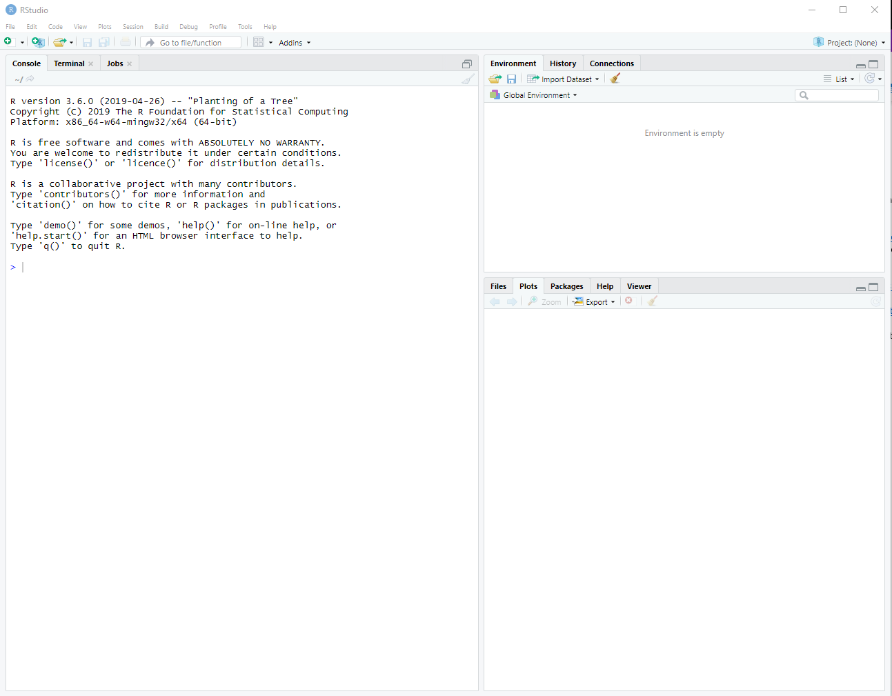
Figure A.1: The Rstudio interface.
If this doesn’t work successfully for you, please reach out and I will help you debug it.
A.4 Using R Markdown Files
Now that R and RStudio are successfully installed, let’s discuss how to crate and use R Markdown files.
When using R, in fact almost all of the work we’ll do this year will be within R Markdown files (within the RStudio environment). In this section we will learn to:
- create a new R markdown file,
- add and run some R code,
- add general descriptive text, and
- then finally “knit” that file into HTML format.
You will typically submit both the knitted *.HTML file along with the raw *.Rmd file to Canvas as evidence of completing your homework.
A.4.1 Creating and Saving Your First *.Rmd File
- To create a new R Markdown file, go to “File -> New File -> R Markdown…” which will open a dialog box. Give it a title, such as “First R Markdown”, add your name as the author, and the press ‘OK’.
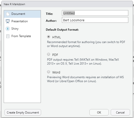
Figure A.2: The New R Markdown file dialog box.
This will create and display a new R Markdown document, which will appear in the upper left of the RStudio work area, above the console.
You should then delete everything in the file below and including “## R Markdown” header, i.e. everything from line 7 on down. You only need to keep the YAML header, lines 1 through 6. The code that you’re deleting in lines 8-30 is just an example.
Next save this file to your computer in an appropriate folder, giving it an relevant name, e.g.
HW0-BL-v1.Rmd, where BL stands for Bert Loosmore and v1 is for version 1. Adding your initials to the end will make it easier for me to review your homework.
I encourage you to use a meaningful file structure on your computer, something like Senior\Fall\Statistics or similar. This will be important as we load and create files. And as we iterate through assignments, you will often have multiple versions of your HW.
Important! - when saving the file to your computer, make sure it has the file extension of *.Rmd. If you don’t save it with the correct extension, it will NOT knit properly.
A.4.2 Editing R Markdown Files
Now let’s edit the R markdown file to use some simple R commands and do some basic probability and statistics. Then we’ll knit to HMTL. I suggest you open RStudio and follow along.
There are two ways we will edit (add content to) R Markdown files: code chunks and descriptive text.
Code chunks are where we write R code and do calculations. These need to be surrounded by the appropriate header and footer, and they appear with a gray background.
The easiest way to create a new code chunk is to type CTRL-ALT-I (all at the same time). This will insert a code chunk at the cursor location and appear as:

Figure A.3: When you create a new R chunck, either by using CTRL-ALT-I or manually, it will appear as shown. Type R commands starting on the blank line in the middle.
You will type all of your R code between the apostrophes, so in what’s shown above this would occur between lines 12 and 14. Just hit RETURN if you need more space to expand the code chunk.
You can also type general, descriptive text outside of code chunks to add any comments or other notes you might want to make. We’ll learn shortly about how we can add formatting to this general text. (For those of you who want a head start on this, here is a resource: https://www.rstudio.com/wp-content/uploads/2015/02/rmarkdown-cheatsheet.pdf.)
For example, you might type “Here is my random data:” before the first code chunk, or “In this plot I observe the data to show a strong linear trend.” after a plot. Statistics is more than just getting the numerical right answer! Most of your submissions will contain a fair bit of descriptive text about what you did and what you observe.
The image below shows an example with both descriptive text (on line 13) and an R code chunk (lines 14-16) in the appropriate places.
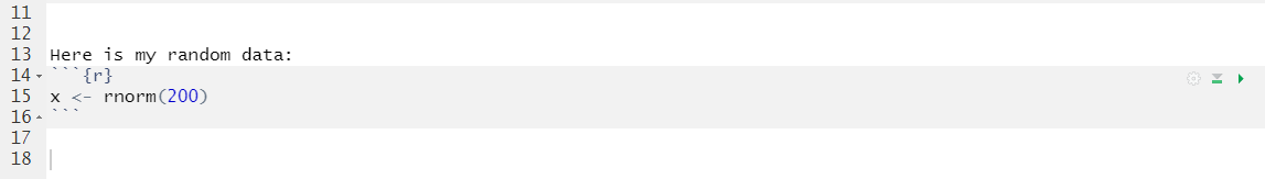
Figure A.4: Executable R code should go within the R chunk. Any comments or supporting text should go outside the R chunk.
In summary:
- Descriptive Text occurs outside the code chunk and includes any description of your work (e.g. how you approached the problem, what you found, etc.)
- Code Chunks contain executable R code, including variables and function. (Code chunks might possibly contain programming comments specific to the R code itself, but more on comments later.)
A.4.3 Our First R Code
Next, let’s do a few things to make sure your system is working and ready for class, and to begin to familiarize yourself with R.
- First, we’ll generate some random data, in this case 200 data points from a Normal distribution (more on what that means later), and then store the results in a variable called
x. Create a new code chunk (remember Ctrl-Alt-I) and then type the following:
After you’ve typed the code above, press the green play button in the upper right corner of the code chunk. What happens?
Well, nothing, or at least nothing that you can immediately see.
This command first generates the 200 random data points and then assigns them to x using the <- (aka ‘gets’) characters. This is actually two characters, the less than < and the minus sign -. In this case, x is not a single valued variable, but a vector, which is a list of 200 different values. Also, the value of 200 is a "parameter" to the built-in rnorm function.
For those of you new to programming, I will explain more details of variables, functions and parameters in our first lab.
(To generate a vector with a different number of random values, we would use a different number. To generate a different type of data, we would use a different function.)
Assuming you typed it correctly, the assignment happens, but you didn’t ask R to display any results, so it didn’t. (Note: R is a programming language and is VERY particular about spelling and syntax.)
- To inspect, or display, your result, just type the name of the variable, in this case
x, which in this case will print out a long stream of data, namely all 200 data points. Again, add this to either a new code chunk (or put it on the line after the variable assignment) and press the green “play” button.
##   [1]  1.138664225  0.374393112  0.900531294  1.499134012 -0.439379442
##   [6]  0.678890895 -0.858574758  2.118773649  1.613919045  1.310922295
##  [11] -0.207886054  0.336377327 -0.421048587  0.274510628  0.606797604
##  [16]  1.448618526 -0.265824642 -0.777111750  0.436186282  0.551905272
##  [21] -1.213266425  0.004542404  0.774320163  0.791202672 -0.522154125
##  [26]  0.942793798 -0.125332124  0.341518584 -0.181995961  2.157177578
##  [31]  0.494446782  0.543756986  0.465032618  0.070309631 -0.273693106
##  [36]  0.042475524  0.352258276  1.334436435  0.321470054 -1.460970423
##  [41] -0.054766708 -0.247756792 -0.307509399  0.140511318  0.506471770
##  [46] -1.728830418  1.099834909  0.064643684  0.812397201  0.922704665
##  [51] -0.437775526 -0.405574505 -1.884810671  0.348234944 -0.365924562
##  [56]  1.404815669  0.886630776 -0.530245977  1.115429736  0.409275706
##  [61]  0.046663992  0.012385300 -1.642057997 -0.468089302  0.457099084
##  [66]  1.007558530 -1.611049239  0.190368269  1.920171452 -0.233863818
##  [71]  0.912760667 -0.087088127 -0.590003248 -0.841364109  0.958271348
##  [76]  0.630646640 -0.559342094 -0.635723047 -0.465686597 -0.606430019
##  [81] -0.572574149 -1.369281851  0.036410632 -0.052113870  2.456277397
##  [86] -0.808943468 -1.350187866 -0.487912083  0.624352320  1.234397777
##  [91] -1.346996207 -0.604802063  0.071614210 -0.218078808 -0.930136051
##  [96] -1.093561592  1.703649925  0.211139718  1.317469329  0.161507606
## [101] -0.305697910 -0.516028751 -0.210548071 -1.149681046  0.661833638
## [106]  0.068108322 -0.553376709  0.614310469  0.163723949  1.389120253
## [111] -0.998371605  0.500669307  1.692965188 -0.950566074 -0.840953339
## [116] -0.213315076 -1.587486183  0.768291874  1.900063513 -1.334982366
## [121]  0.520674101 -0.691075554 -0.418391234  0.473267490  1.331279792
## [126] -0.688280813 -0.030682792  1.207199348 -2.098270755 -0.517969338
## [131] -0.587552514 -1.605021386  1.391335886 -0.595118528  1.219905214
## [136] -1.374225386 -0.676887242 -0.091261318  1.324767691 -0.320396474
## [141] -0.763165963  0.541781730 -1.265534985 -0.567831096  0.269381303
## [146] -0.267049942 -1.110712580  0.285851163  0.940202572 -2.027974669
## [151] -0.462999483 -0.868624948  0.581481406  0.036132138 -1.785266556
## [156] -0.366320119 -0.733109621 -0.539099161 -0.439539030 -1.313402002
## [161]  0.200989431  1.046628631 -1.313218744  0.635983762 -0.315012200
## [166] -0.782921689 -1.513248474 -0.776224738  0.242170213  1.127270287
## [171]  1.513212003 -0.201016437 -0.809464453 -0.587910136  0.125964659
## [176]  0.001363162 -1.688087609 -1.088675714  0.920363959  0.907798023
## [181]  0.278519066  1.358977244  0.390584944  0.596037827  0.824846831
## [186]  1.750831545 -0.180670598 -0.733496125 -0.557676939 -0.379419106
## [191]  1.329250727  0.648923255  1.355006467 -1.156764052 -0.918287950
## [196]  0.195967234  0.292193903 -0.313070493  0.586451241 -0.280388783
If that worked, you should now see a list of 200 numbers.
Next, let’s use R to calculate the average or mean of our data. Create a new code chunk and type and execute the following (remember to press the green arrow):
## [1] 0.02026349When you press the green arrow, R should print out the mean value. Note, because of randomness your value will likely be different than mine.
- Next, let’s plot the data, using the following command, again within a code chunk.
After running this code chunk, your plot should look something like mine, although again since the data values are random, your plot should not be exactly the same.
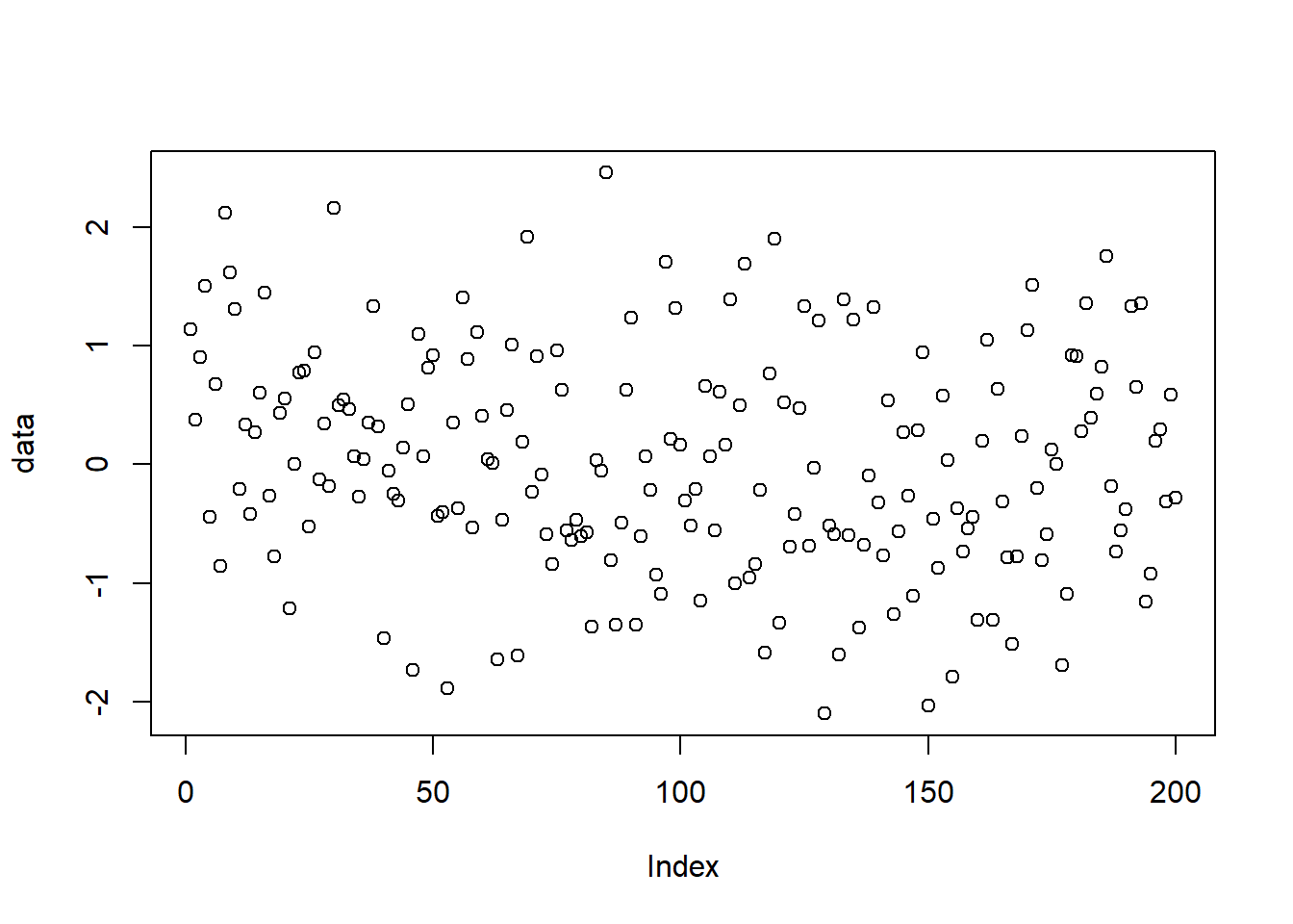
Here, the vertical (y) axis is the data value from our simulation, and the horizontal (x) axis is the index, or simulation number. Remember, we simulated 200 points? Hence there are 200 values plotted.
- We’ll spend a lot of time this year evaluating data and plots. Some questions we might ask here include:
- What does this data show?
- Do you see any patterns?
- Do the values seem random?
- Do they seem constrained in anyway?
- What would you guess the mean is?
Above I mentioned we can add general text to R Markdown files. To complete this warm up, answer one or two questions of your choice, adding descriptive text below your plot, OUTSIDE of a code chunk.
When you knit, this text will come across as text.
And, if you get this far, you’re done with the basic calculations! Now on to knitting.
A.4.4 Knitting your File to HTML
In this next step, you will attempt to convert your R markdown into a nicely formatted HTML file. RStudio makes this pretty easy to do.
- In fact, this should be as simple as pressing the knit button, as shown below.
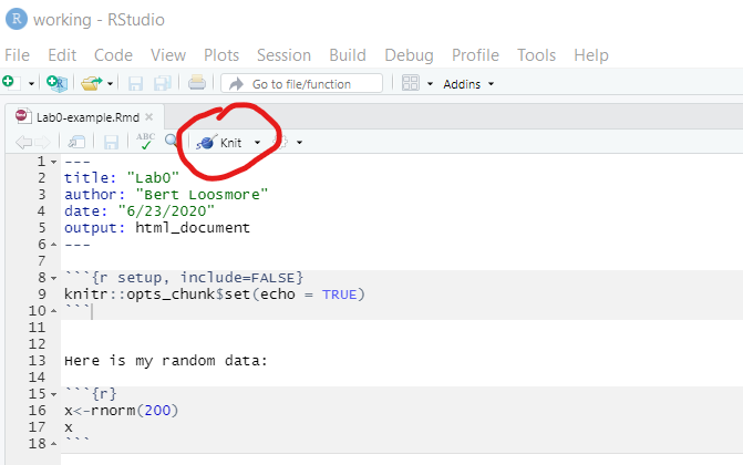
Figure A.5: The location of the Knit button is shown in the red circle. Use this button to create an *.html file output.
RStudio will run for a few seconds and then generate an HTML file. (Note: The first time you attempt to knit a file, R may ask you to install a couple of additional packages. You should install these, just follow the directions on the screen.)
If my file was called HW0-BL-v1.Rmd, then my knitted result would be HW0-BL-v1.html, and is located in same folder where you saved your *.Rmd file.
- Open and inspect your HMTL file. Double clicking it should open it in your default browser.
What do you notice? Generally it should look similar to the HTML file where the lab was created. There are code chunks in gray and plain text in white. Code chunks should display both the code and the results.
That’s it! For most HW assignments I will ask you to submit both the *.Rmd and *.html files to Canvas. (No need to submit anything here.)
Congratulations! Your RStudio installation is working and you’re well on your way to becoming proficient in R.