Chapter 13 Experimental Design

13.1 Overview

The goal for this chapter is to introduce the concept of Experimental Design. We’ve spent a significant amount of time discussing HOW to run hypothesis tests, but those results are only valid IF the experiment or observational study was set up (i.e. designed) correctly. Here, we’ll focus on what comprises proper experimental design.

There is a lot of terminology in this chapter, some of which should be familiar, and after working through those definitions, we will then examine some different scenarios to discuss what might be good and bad examples.

After this unit you will have the opportunity to design (and possibly execute) your own experiment and analyze the associated data.

13.1.1 Learning Objectives

After this chapter, you should be able to:

Describe the types of questions that “statistical analysis” can answer
Identify the population and the sample of a given statistical question, and discuss how knowing the population of inference informs how the sample should be taken
Explain what a random sample is and how it relates to statistical inference
Identify the experimental unit, treatment, and response for a given statistical study
Identify possible confounding variables for an experiment
Define explanatory and response variables, and explain the need for knowing the type of test to be run BEFORE the experiment is started.
Explain the meaning of the terms control group, placebo-effect and double-blind, as well as their role in statistical experimentation
Explain the difference between an observational study and experiment
Name and explain some types of bias that can occur during sampling, and understand the impact that bias can have on our conclusions (i.e. that they can effect both the mean and standard error estimates and so invalidate our results!)
Describe what a simple random sample is and when it is appropriate.
Understand the four (4) components of a well designed experiment
Define type I and type II errors
Explain what the terms \(\alpha\), \(\beta\) and statistical power mean
Calculate the type I and type II error rate for a given \(H_0\) and specific \(H_A\)
Describe how and why \(n\) (sample size) is one of our best levers for controlling our type II error rate in hypothesis testing

As long as it is, this list of terms related to experimental design is NOT comprehensive. There are often multiple components to proper statistical design, depending on the details of the hypothesis test being run, for example. The intent of this chapter is to provide an overview of the key concepts.

13.2 What types of questions can statistical analysis answer?

Compare the following two questions:

What was the high temperature at EPS, measured on the fourth floor balcony on May 1st, 2020?
How does the average high temperature in Kirkland in May 2020 compare to May 1990?

One of these needs statistical analysis (and evaluation of the uncertainty) to be answered, while the other can be answered directly with proper measurement.

For the first question, we can measure that explicitly. It has a specific location and time. There is a single answer.

The second question, on the other hand, did not specify the exact location (where in Kirkland?) and is asking about the average value. That implies we may need to take multiple samples across different locations for both dates (we can’t feasibly measure all of Kirkland) and that we will be comparing both the average value and standard deviations.

The point is that we only use “statistical analysis” when either (i) we aren’t able to sample the entire population or (ii) an evaluation of uncertainty is required.

This then leads to needing to understand how we should design our experiments so that the results are valid.

13.3 The Components of Experimental Design

13.3.1 Samples vs Populations

We’ve talked about a sample as being a set of measurements from a subset of the larger population of interest. A sample should be randomly selected, with the goal of accurately representing the opinions or data from the larger group.

Why does it need to be random? To ensure it is truly representative of the population.

As such, it is important to be clear about the population about which you want to make inference, and then choose the sample accordingly.

If we think about the effectiveness of the COVID-19 vaccine, we are certainly concerned about whether it provides effective coverage to all who receive it. However, since different demographics (such as age) seem to respond differently to the disease, in designing an experiment to test efficacy, we may want to be more specific about the target population, whether that is based on age, race, geography or other.

One of the concerns early on in vaccine development and testing was that not enough PoC were included in the initial trials. If they weren’t, the potential inference would be flawed. Hence it is critical to make sure the sample and population line up.

As another example, if we are interested in some characteristic of EPS students, but only interview boys, our inference will be invalid.

Even with random sampling, our sample may not be representative of the target population.

For example:

Is randomly sampling EPS students representative of WA high school students? Why or why not?
Is randomly sampling Seattle voters representative of WA state voters? Why or why not?

In all cases it may be that the answer is “it depends”. For example, if you ask a certain population about gun control rights, the question of how representative your sample is may be different than if you ask the same group about the value of public lands for recreation.

13.3.2 Why is a Random Sample important for Statistical Inference?

Once we’ve chosen the population, we need to make sure the sample is randomly selected from the population in order to try to control any type of bias. We will discuss types of bias in further detail below.

See the Gettysburg Address class activity.

13.3.3 Experimental Units, Treatments, and Responses

Generally, when we think about an “experiment”, we probably think about testing two different processes or groups, measuring what happens, and then comparing the result.

To put this into statistical speak, let’s define a few terms:

The experimental unit describes the subject that the experiment is happening upon. This could be people, communities, plants, plots of land, solutions (liquids), etc.

The treatment describes the specific (set of) experiments being run on each group of experimental units. It might be the dosage (or placebo) administered. It might be the combination of the type of variety of plant planted along with the amount of fertilizer applied. There are typically at least two treatments being compared within an experiment, possibly as a treatment compared against a control group.

In general, there are more than one experimental unit within each treatment group to increase our statistical power. More on that later.

The response is the quantitative (or possibly qualitative) variable we are measuring on each experimental unit to track the effect of the given treatment. It could be weight, height, growth, a measure of health, or other.

So, putting these three together, to run an experiment, we divide our sample into multiple groups, each group containing a number of experimental units. Each experiment unit then receives one of the treatments and is measured for the response. (Of course we might measure the experimental unit both before and after the treatment is applied.)

13.3.4 An Example

Imagine a scenario to increase voter engagement where we want to test whether phone calls and/or mailers have an effect. A possible experiment might:

take a random sample of the population of interest
divide the sample into three groups
do nothing with the first group, call the second group to remind them to vote, and send mailers to the third group to encourage them to vote
measure the voting rate of all three groups separately
compare the results (such as via ANOVA which we will learn in a later chapter)

Here the experimental unit is a person. The treatment is either: do nothing, call, or send mailer. The response is whether they voted.

Of note, it is important here that we have a control group (where we do nothing) so we can tell if the differences in voter engagement are related to our treatment(s) or possibly some other (confounding) variable that impacts all groups. What are confounding variables? More on that in the next section.

13.3.5 Confounding Variables

A confounding variable is one that is included (possibly unintentionally) within our experiment that causes potential issues with our analysis. For example, let’s suppose we are measuring efficacy of the COVID-19 vaccine, and have two groups we are studying (vaccine vs. placebo). Now let’s imagine that our experimental design did not account for a patient’s wealth when we did our random selection, and a disproportionate number of higher wealth individuals were in the placebo group.

Since wealth and lifestyle might have a significant impact on outcomes, if we don’t account for it, it might confuse (confound) our results.

In particular, if the group that is given the treatment also has more wealthier individuals and has better outcomes, (however we define that), do we attribute it to the treatment or their wealth? And more troublesome is that if we don’t consider wealth at all in this example, we won’t know if such confounding occurred.

13.3.6 What will you do with the Results?

An important (critical) part of the experimental design process is to think through how you will analyze the results, and to do this BEFORE collecting any data. This accomplishes at least two things:

ensures that you’ve thought about the likely explanatory variable, possible confounding variables and other sources of bias
confirms that the type and form of the data you’re collecting can be analyzed based on your chosen statistical methods

The explanatory variable describes the treatment that we expect or is being investigated to have a statistically significant impact on our response. If both your treatment and response were continuous variables, you would probably create a scatter plot f your results, and then you might think of this being our \(x\) variable with the response being our \(y\) variable.

If we only have one treatment group (vs. control), the treatment and explanatory variable are often the same. Where we have different treatments and/or multiple treatments, the experimenter should be clear about which is the potential explanatory variable.

13.3.8 Experiments vs. Observational Studies

Above we described the components of an experiment and in fact there is another type of design that statistical analysis applies to: observational studies.

The key difference here is whether the experimenter is manipulating anything or applying “treatments” to the experimental unit (the subject being evaluated). If not, (i.e. if the experimenter is simply observing the two groups), then this is known as an observational study.

Observational studies can either be retrospective (looking at previous results) or prospective (looking and current and future results). Each has advantages and disadvantages.

Generally experiments are better able to control for bias and have better statistical power than observational studies. However, in some cases, we can only perform observational studies, particularly in cases where people’s health might be at risk. For example, we wouldn’t randomly assign people to be exposed to second hand smoke or not.

13.3.9 More on Types of Biases

Bias occurs when certain responses are systematically favored over others, and are often the result of poor experimental design. Some examples of types of bias include:

Voluntary response bias occurs when a sample is comprised (entirely) of people who choose to participate, such as those people with strong opinions (and hence the sample won’t typically be representative of the whole population).
Undercoverage bias occurs when part of the population (by demographic, for example) has a reduced chance of being included in the sample but does exist in the overall population (and hence the sample won’t typically be representative of the whole population). A typical example of this is only attempting to contact people via land-lines (telephones).
Quota sampling bias occurs when interviewers are allowed to choose the participants or specific experimental units in the sample, in an effort to make it representative. Don’t!
Nonresponse bias occurs when data from individuals chosen to be sampled cannot be obtained (maybe they refuse to respond), AND whose results may differ than those who do respond.
Question wording bias occurs when problems in the survey result in incorrect responses. This could result from confusing or leading questions.

Non-random sampling methods also introduce the potential of bias.

What happens if we have bias in our sample? Our data will be off and potentially not representative of our population. This could impact our estimates of both the mean \(\bar x\) and the standard deviation \(s\) of our sample, which can invalidate both our inference and hypothesis testing results.

13.3.10 Sampling Methods

Given that we need to be careful about bias when designing our experiment, how should we proceed?

First, it is important to think about potential sources of bias and possible confounding variables BEFORE we start collecting data.

The basic approach is to collect a simple random sample (SRS). If the whole population is available to us, we can use a random number generator to choose our sample. The sample() function in R makes this easy. Under this approach, each individual in the population is equally likely to be included in our sample.

However, this is only appropriate if our population is homogeneous. Otherwise, confounding variables may cause us problems, particularly where our random selection causes a confounding variable to be disproportionately included in one group compared to the other.

To solve this issue we might use a more advanced sampling techniques:

First, we might use a stratified random sample. This involves first sub-dividing the population into potentially important groups (location, age, race, wealth, sex, etc.), then randomly sampling from each group or strata, and finally either combining across strata into your two (or more) samples to evaluate, or keeping separate as appropriate. In the latter case, you would have more than 2 groups to evaluate, and this allows for determining if the differences across strata are statistically significant.

Alternatively, we may be more interested in characterizing the variability that exists within groups, and less interested in the exact causes. For example, what is the average streaming service (e.g. Netflix, Amazon Prime, Disney+, etc.) usage among in cities in the Seattle area compared with the NY area? In this case, while I know there are differences and variability among individual households, we are more interested in how cities compare. In this case, I’ll use cluster sampling, where we divide the population in each region into heterogeneous groups, and our random sampling consists of which specific groups (e.g. cities) we select and measure.

As we have seen and will continue to discuss, our ability to distinguish between groups is driven by the amount of variability present. A stratified random sample works to remove this variability whereas a cluster sample preserves it. So, back to our streaming services example, if the within city variability is high, we won’t be able to easily distinguish different regions.

In summary the type of sampling you choose depends a lot on the research question you’re asking and your population of interest. Often we’ll take so some preliminary measurements and perform some EDA (exploratory data analysis) to get an understanding of the type of variability that exists in our population, and this can help guide further sampling approaches.

13.4 What Constitutes a Well-Designed Experiment?

Now that we have discussed all the details of what might go into an experiment, how should we set it up?

There are four components of a well designed experiment, including:

Comparisons of at least 2 treatment groups, one of which could be a control group
Random assignment of treatments to experimental units (participants or subjects)
Replication, meaning (i) more than one experimental unit in each group and (ii) should be able to be reproduced by others
Control of potential confounding variables and reduction of bias where appropriate

13.4.1 Guided Practice: Read the Sample Experiment

Imagine the following experiment:

We want to test whether listening to music or white noise while studying leads to improved learning and retention. We select 30 students and randomly sort them into two groups. Each group is given a list of 25 vocabulary words to memorize and instructed to study for 15 minutes per day for a 1 week period. The first group is allowed to listen to music during their study time and the second group is required to listen to white noise during their study time. After 1 week, each group is tested on their knowledge and receives a score between 0 and 100.

For this experiment, identify and/or define the following as best as possible. If information is missing, suggest what might be appropriate.

What are the experimental units? What are the treatment(s)? What is the response?
For what population is the inference appropriate? How is the sample being taken? How are the treatments assigned?
Are there any potentially confounding variables that are or are not accounted for? How might you modify the design to reduce their impact?
What other possible sources of bias might exist?
Does this experiment use a control group? Is this an example of a double-blind experiment?
Is this an observational study or an experiment?
Are the four (4) components of a well-designed experiment included? (if so explain how, if not explain how you might modify the design)
What statistical method would you use to evaluate the data?

Again, if you need to add (make-up) details that aren’t included above to answer the above questions, please feel free to do so.

13.5 Type I vs. Type II errors

When we previously talked about \(\alpha\) and determining critical values we acknowledged that even when our test statistic exceeded our critical values (either below the lower or above the upper) there was still some finite probability of the test statistic having come from the null distribution simply based on randomness.

Is it therefore possible we might reject \(H_0\) when in fact \(H_0\) is true?
And similarly, could we fail to reject \(H_0\) when in fact \(H_A\) is true?

In this section we will explore these questions.

13.5.1 Learning Objectives

By the end of this section you should be able to:

Define type I and type II errors
Explain what the terms \(\alpha\), \(\beta\) and statistical power mean
Calculate the type I and type II error rate for a given \(H_0\) and specific \(H_A\)
Describe how and why \(n\) (sample size) is one of our best levers for controlling our type II error rate in hypothesis testing

13.5.2 Mistakes in Hypothesis Testing

So, what is the probability we reject \(H_0\) if in fact \(H_0\) is true? How would we quantify this? (You should be able to figure this out, draw pictures if necessary and brainstorm this with your table mates.)

As a hint: you will reject if \(\hat p\) or \(\bar x\) (or our test statistic) is outside the critical values. What is the probability outside the critical values?

.
.

I introduced a new concept here, namely what is “true”. In fact we have both the truth AND we have what our test tells us. Importantly, these may or may not be the same.

And note, if this happens (i.e. if we reject \(H_0\) when \(H_0\) is true), we’ve made a mistake, an error.

Let’s talk more about the what the truth might be and what our test conclusion might be. The following table shows the four outcomes that could occur. The rows indicate the truth and the columns indicate what our test conclusion is.

types of errors	Reject \(H_O\)	Fail to reject \(H_0\)
\(H_0\) is false	correct	error
\(H_0\) is true	error	correct

.
.
.
.

From above, we realized that the probability of rejecting \(H_0\) if \(H_0\) is true is \(\alpha\). But what about the probability that you fail to reject \(H_0\) if \(H_A\) is true? This would also be an error.

To answer this question, we need to know more about \(H_A\). Here we’re going to modify how we think about \(H_A\) in that we’ll assign a specific value. This is because the probability that you fail to reject \(H_0\) if \(H_A\) is true depends on the distribution of \(H_A\).

Imagine the following scenario where we have \(H_0: \mu = 80\) and where we’ve quantified the distribution of \(H_A: \mu =65\).

x <- seq(from=40, to=100, by=0.25)
y <- dnorm(x, 80, 5)
plot(x,y, type="l")
lines(x, dnorm(x, 65, 5), col="blue")
cv = qnorm(0.05, 80, 5)
# abline(v=cv, col="red")
text(90, 0.06, "HO")
text(54, 0.06, "HA", col="blue")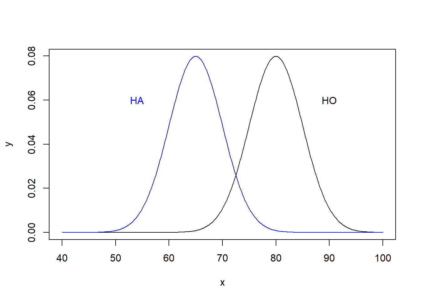

Note that when (and only when) we quantify a specific \(H_A\), can we then answer our question. Importantly, observe the overlap that exists between the distributions.

I’ll now add the lower critical value at \(\alpha=0.05\) assuming a 1-sided test for \(H_0\). These means 5% of the distribution of \(H_0\) is below the red line.

x <- seq(from=40, to=100, by=0.25)
y <- dnorm(x, 80, 5)
plot(x,y, type="l")
lines(x, dnorm(x, 65, 5), col="blue")
cv = qnorm(0.05, 80, 5)
abline(v=cv, col="red")
text(90, 0.06, "HO")
text(54, 0.06, "HA", col="blue")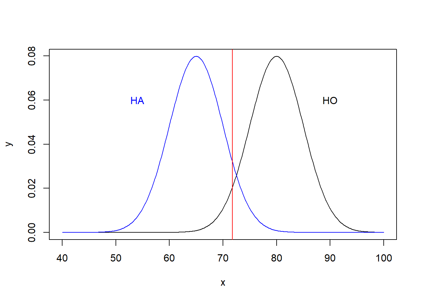

Now, let’s ask: What is the probability of failing to reject \(H_0\), if \(H_A\) is true?

Let’s break this question down. How would we fail to reject \(H_0\) in the above diagram? If \(\bar x\) (our test statistic) is above the critical value, in this case 71.77 (the red line).

qnorm(0.05, 80, 5)

## [1] 71.77573

However, note, for this question here we’re assuming \(H_A\) is true. So, what is the probability above the critical value under the \(H_A\) distribution? We can find this as:

pnorm(qnorm(0.05, 80, 5), 65, 5, lower.tail=F)

## [1] 0.08768546

or 8.79%.

So, for this specific value of \(H_A: \mu = 65\), there is a roughly 9% chance of making the error where we fail to reject \(H_0\) when in fact \(H_A\) is true.

This probability would change for different values of \(H_A\), in particular it would increase as \(H_A\) gets closer to \(H_0\) and would decrease as \(H_A\) gets farther away from \(H_0\).

This should make some sense. Our power to reject a given \(H_A\) depends on how close or far that value is from \(H_0\).

13.5.3 Defining Type I and Type II Errors

Above we talked about two types of errors we might make during hypothesis testing. Namely we make a mistake when we either:

reject \(H_0\) when it is true, or
fail to reject \(H_0\) when \(H_A\) is true,

We’ll call the first one a “Type I” error and the second one a “Type II” error. Going back to our table:

Types of errors	Reject \(H_O\)	Fail to reject \(H_0\)
\(H_0\) is false	correct	Type II error
\(H_0\) is true	Type I error	correct

As we discussed above, \(\alpha\) is the probability of a type I error. We’ll use \(\beta\) to represent the probability of a type II error, and we’ll often use the term the power of the test where we define Power = 1- \(\beta\).

Remember, that we can always calculate our type I error (since this is just \(\alpha\)), however we can only calculate \(\beta\) for a specific \(H_A\).

13.5.4 Adjusting \(\alpha\), \(\beta\) and \(n\)

So, what can we do to minimize our errors? Obviously our choice of \(\alpha\) is important here. Why not decrease it beyond 0.05 to make fewer type I errors?

As we’ve seen, when we decrease \(\alpha\), our critical values push out wider. Inspect the graphic above and consider what would happen to \(\beta\) as this occurred. Everything else held constant, more of \(H_A\) would then fall to the right of the critical value, which would increase our type II error rate.

Hence, there’s an important trade off between \(\alpha\) and \(\beta\). If we decrease our type I error rate, our type II error rate will increase.

A little later we’ll discuss in more detail how sample size (\(n\)) impacts these error rates, and to introduce that idea here, remember that sample size impacts SE, which widens or narrows the two distributions above and therefore changes both:

the location of the critical value for \(\alpha\) and
the percentage of \(H_A\) within the acceptable range of \(H_0\) (i.e. within the critical values).

The point of this is that by choosing the sample size thoughtfully, we can adjust the power of the test against a specific \(H_A\). Generally, this is the most important lever we have, assuming we’ll keep \(\alpha=0.05\).

13.5.5 Simulating type I error rates

Just to reinforce the point, let’s run a simulation to prove that \(\alpha\) is the type I error rate.

Assume \(H_0: \mu \ge 80\) with \(SE=5\) (as above). Here we’ll again assume a 1 sided test.

First, a little background and let’s imagine what our initial population might be. For example, the following scenario (i.e. \(\sigma=50\) and \(n=100\)) leads to as standard error of 5.

sigma <- 50
n <- 100
se <-sigma/sqrt(n)
se

## [1] 5

Next, let’s calculate our critical value:

cv <- qnorm(0.05, 80, 5)

Now let’s draw 10000 samples of 100 responses from our initial population using rnorm(). For each we’ll calculate \(\bar x\). Finally, we’ll calculate what percent of those are below our critical value.

a <- vector("numeric", 10000)

for (i in 1:10000) {
  b <- rnorm(100, 80, 50)  # this is the sample of n=100 from our initial population 
  a[i] <- mean(b)          # this is the corresponding estimate of x-bar
}

length(which(a<cv))/10000

## [1] 0.0496

which we see is very close to \(\alpha\). In every one of those cases, our test statistic would have been below the critical value and we would have incorrectly rejected \(H_0: \mu = 80\).

13.5.6 Review of Learning Objectives

By the end of this section you should be able to:

Define type I and type II errors
Explain what the terms \(\alpha\), \(\beta\) and statistical power mean
Calculate the type I and type II error rate for a given \(H_0\) and specific \(H_A\)
Describe how and why \(n\) (sample size) is one of our best levers for controlling our type II error rate in hypothesis testing

13.6 Review of Learning Objectives

After this chapter, you should be able to:

Describe the types of questions that “statistical analysis” can answer
Identify the population and the sample of a given statistical question, and discuss how knowing the population of inference informs how the sample should be taken
Explain what a random sample is and how it relates to statistical inference
Identify the experimental unit, treatment, and response for a given statistical study
Identify possible confounding variables for an experiment
Define explanatory and response variables, and explain the need for knowing the type of test to be run BEFORE the experiment is started.
Explain the meaning of the terms control group, placebo-effect and double-blind, as well as their role in statistical experimentation
Explain the difference between an observational study and experiment
Name and explain some types of bias that can occur during sampling, and understand the impact that bias can have on our conclusions (i.e. that they can effect both the mean and standard error estimates and so invalidate our results!)
Describe what a simple random sample is and when it is appropriate.
Understand the four (4) components of a well designed experiment
Define type I and type II errors
Explain what the terms \(\alpha\), \(\beta\) and statistical power mean
Calculate the type I and type II error rate for a given \(H_0\) and specific \(H_A\)
Describe how and why \(n\) (sample size) is one of our best levers for controlling our type II error rate in hypothesis testing

13.7 Exercises

Exercise 13.1 A company wants to compare two washing detergents (Brands A and B) to see which best keeps colors from fading. Twenty new, identical red t-shirts will be used in the trials. Ten t-shirts are washed 15 times with Brand A in warm water. The other 10 t-shirts are washed with Brand B in cold water. The amount of fading is rated on a 0 to 100 scale, and the mean for the t-shirts washed in Brand A is compared to the mean for the others.

What are the population and sample? What is the treatment? What is the response?
Do you think this a good experimental design? Why or why not? Make sure to discuss both (i) what is good, and (ii) what could be improved.

Exercise 13.2 Jillian wants to know what percent of students at her school watch sports on TV. Which strategy for sampling (a or b) will be more likely to produce a representative sample? For your each option below identify the population for which inference would be appropriate.

At the next school football game, she asks every third student who enters whether or not they watch sports on TV.
At the next school assembly, she ask every third student who enters whether or not they watch sports on TV.

Exercise 13.3 David hosts a podcast and he is curious how much his listeners like his show. He decides to start with an online poll. He asks his listeners to visit his website and participate in the poll. The poll shows that 89%, percent of the 200 respondents “love” his show. What types of bias exist in his result? How could he reduce this?

Exercise 13.4 A senator wanted to know about how people in her state felt about internet privacy issues. She conducted a poll by calling 100 people whose names were randomly sampled from the phone book (note that mobile phones and unlisted numbers aren’t in phone books). The senator’s office called those numbers until they got a response from all 100 people chosen. The poll showed that 42% of respondents were “very concerned” about internet privacy. What types of bias (if any) exist in this result?

Exercise 13.5 Explain why a double blind experiment is useful? Under what conditions (situations) do you think it is necessary? Describe a situation when it can’t be used.

Exercise 13.6 Twenty men and twenty women with migraine headaches were subjects in an experiment to determine the effectiveness of a new pain medication. Ten of the men and 10 of the women were chosen at random to receive the new drug. The remaining men and women received a placebo. The researchers did not know which patients were given which pill (drug or placebo). The decrease in pain was measured for each subject.

What are the experimental units? What are the different treatments? What is the response variable?
Is this an example of a double blind experiment? Why or why not?
What are some possible confounding variables?

Exercise 13.7 Describe how you would create an observational study to evaluate at whether there is an effect of screentime on spinal health in teens. Be clear about your sample and population, how you would create your groups and what you would measure. Why should or shouldn’t this be conducted as an experiment?

13.7.1 Type I and Type II errors

Exercise 13.8 Consider a two-sided hypothesis test run at the \(\alpha = 0.05\) level.

What is the probability of a type I error?
If the null distribution is \(H_0: \mu = 25\) with \(SE = 5\), plot the distribution and add vertical lines to indicate where type I errors occur.
Now consider an alternative hypothesis of \(H_A: \mu = 18\) (also with \(SE= 5\)). Add this distribution to your plot from part b, and you might consider a different color for the line. Based on the critical values from part b, what is the probability of making a type II error?
Finally consider an alternative hypothesis of \(H_A: \mu = 15\) (also with \(SE= 5\)). Again based on the critical values from part b, what is the probability for this \(H_A\) of making a type II error?.

Exercise 13.9 Consider a two-sided hypothesis test run at the \(\alpha = 0.05\) level, with \(H_0: \mu=18\), a population \(\sigma = 6.2\) and \(n=100\).

What is the standard error?
What is the power against an \(H_A: \mu = 20\)? Remember power is \(1-\beta\).
If you instead sample \(n=400\) people, how does your answer to part (b) change?

Statistics at Eastside Prep