Chapter 8 Discrete Probability Distributions
8.1 Overview
So far we’ve talked a fair bit about probability, including rules and how to do certain calculations. For the most part we’ve dealt with events where there were on a few discrete possible outcomes, e.g. “H” or “T” or colors of Skittles.
In this chapter, we stay with discrete random variables and introduce the idea of discrete probability distributions, and in particular those which have an analytical form.
In general, probability distributions describe all of the possible outcomes for a given random variable as well as their associated probabilities. The ones we will discuss here can be written in equation form or visualized like histograms. Since probability distributions describe all possible outcomes, they must sum to exactly 1. Maybe obviously, discrete probability distributions are based on random variables that have discrete outcomes.
The probability distributions we’ll study here include:
- the discrete uniform distribution,
- a Bernoulli trial, and
- the Binomial distribution.
These distributions all have nice mathematical forms, which are characterized by their parameters. For each distribution, we will discuss situations where it is typically used, the parameters used to characterize it, and its mean and variance. We will also discuss functions in R that can be used to simulate data from and evaluate probabilities of each of these distributions.
Finally, we will introduce the concept of cumulative distributions, useful for calculating the probabilities associated with a set of outcomes.
8.1.1 Learning Objectives
By the end of this chapter you should be able to:
- Define the discrete uniform distribution, a Bernoulli trial, and Binomial distribution and describe a situation where each might be applicable
- Define what is meant by a parameter of the distribution.
- List the parameters of the three above distributions and explain the impact of the parameter values on the distribution’s shape and therefore resulting probabilities
- Sketch (by hand or in R) the shape of each of these distributions
- Calculate the mean (\(\mu\)), variance (\(\sigma^2\)) and standard deviation (\(\sigma\)) for each of the above distributions
- Simulate random outcomes (using R) from each of the above distributions
- Calculate the probability density \(P(X=x)\) for each of the above distributions, both by hand and using the built-in R functions
- Explain what a cumulative distribution function is, i.e. \(P(X\le x)\), why it's important, how it’s used, and how to calculate it (in R or by hand) for each of the above distributions. Describe the end behavior of the cumulative distribution.
8.2 The Discrete Uniform Probability Distribution
Let’s suppose you’re interested in designing a new board game and you want to make the probabilities of players winning fair but challenging. What are the probability distributions associated with a 4 sided die or a 20 sided die? You might recognize that these are similar and just differ by the maximum number.
We’ve talked a fair bit about rolling dice, and now let’s consider the probability distribution of the outcomes.
As a reminder, probability distributions:
- contain all possible outcomes and show how likely (probable) each one is, and
- must sum to exactly 1.
For a six sided die, there are six possible outcomes, each with probability 1/6, and so here (not surprisingly) is a visualization of the probability distribution for a single roll of a six-sided fair die.
a <- rep(1/6, 6)
barplot(a, names.arg=seq(1:6), ylim=c(0,1), xlab = "Die value", ylab="Probability")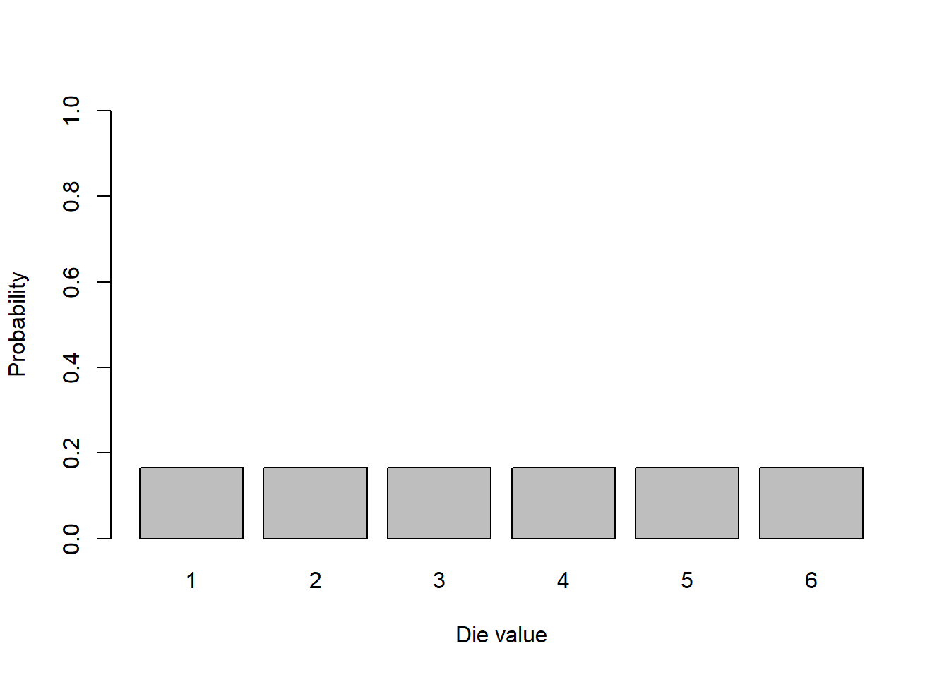
Typically when plotting a distribution we’ll show the outcomes on the x-axis and the probabilities on the y-axis.
As said, this is an example of a discrete uniform distribution. This means the outcomes are discrete and the probabilities of choosing between any of them is equal, or “uniform”.
8.2.1 Our general framework
Going forward, for each of the distributions we’ll encounter here and in the next chapter, I’ll try to answer the following questions:
- What does the graph of the distribution look like? (and don’t worry, they’ll get a bit more interesting)
- What are the parameters for the distribution?
- What are the mean and variance of the distribution?
8.2.2 Parameterizing the Discrete Uniform Distribution
Since the probabilities are all the same, all we need to know to fully describe (i.e. parameterize) the discrete uniform distribution is how many options there are and where they range between. In fact its as simple as knowing the minimum and maximum values. To characterize our single roll of a six-sided die, all we need to know is the minimum is 1 and the maximum is 6. (We assume then that all intermediate values are possible outcomes.)
More generally we will let \(a\) be the minimum and \(b\) be the maximum of the distribution. So in the six sided die case, \(a=1\) and \(b=6\).
8.2.3 Expected Value and Variance
What are the mean (expected value) and variance for this distribution? Actually, we did this already in a previous chapter:
For the expected value of \(X\) we have:
\[E[X] = \sum X_i P_i = 1*\frac{1}{6}+ 2*\frac{1}{6}+ 3*\frac{1}{6}+ 4*\frac{1}{6}+ 5*\frac{1}{6}+ 6*\frac{1}{6} = \frac{21}{6} = 3.5\]
And for the variance, we first have to calculate the expected value of \(X^2\), namely \(E[X^2]\) as
\(E[X^2] = \sum X_i^2 P_i = 1^2*\frac{1}{6}+ 2^2*\frac{1}{6}+ 3^2*\frac{1}{6}+ 4^2*\frac{1}{6}+ 5^2*\frac{1}{6}+ 6^2*\frac{1}{6} = \frac{91}{6} = 15.1667\)
and then use this to find \[Var[X] = E[X^2] - (E[X])^2 = 15\frac{1}{6} - 12\frac{1}{4} = 2 \frac{11}{12}\]
Note the expected value falls right in the middle of the range of outcomes.
Of course, a discrete uniform distribution could have more than 6 options. Many dice games do!
Btw, those of you who are interested in designing or playing diced based board games might find this link from boardgamegeek.com about mean and variance useful.
8.2.4 Using the Parameters of the Discrete Uniform
Now let’s calculate the mean and variance based on \(a\) (the minimum) and \(b\) (the maximum) values. For the discrete uniform we have:
\(E[X] = \frac{a+b}{2}\)
and
\(Var[X] = \frac{(b-a+1)^2-1}{12}\)
So, for our 6 sided die example, \(a=1\) and \(b=6\). We then find \(E[X] = \frac{7}{2}=3.5\) and \(Var[X] = \frac{(6-1+1)^2-1}{12} = \frac{35}{12}\) matching our results from above.
I’ll leave these to you to prove these two results, which you could do using our previous methods for expected value and variance calculations. Those of you with strong math backgrounds might find it a fun challenge.
8.2.5 Simulation in R
What about simulating data in R? We’ve actually done this already. As a reminder, if I wanted to simulate 10 rolls of a six sided die, I would use:
## [1] 5 3 1 2 1 3 6 5 2 2Can you see where the minimum and maximum parameters show up?
8.2.6 Calculating Probabilites
For any individual value, the \(P(X=x)\) (i.e. the probability that a random variable \(X\) takes a specific value of \(x\)), we calculate this as \(\frac{1}{b-a+1}\). It doesn’t matter what the value itself is, because it’s uniform!
(In distributions we’ll discuss soon, the value of \(x\) will affect it’s probability.)
What if we wanted to know the probability of rolling a 3 or greater, written as \(P(X\ge 3)\)? This is another type of question we’ll commonly ask of our probability distributions.
To answer this we simply add up the probabilities of the individual values between 3 and 6. Since all probabilities are equal and there are 4 values, its simply 4*1/6 = 0.67.
You might recognize that it is also the # of values in our set divided by the total # of values in the probability distribution. Or equivalently the # of values in our set times the probability of any given value.
The second term in both cases is \(\frac{1}{b-a+1}\).
Later, when we get to continuous distributions we’ll refer to this calculation \(P(X\ge x)\) (this summing of values) as finding the cumulative probability density (or possibly the “area under the curve” for those who have taken calculus.)
8.2.7 Review and Summary
After this (short) section you should be able to:
- Describe the Discrete Uniform Distribution, including its mean and variance and how to parameterize it
- Calculate its expected value and variance based on the parameter values
- Simulate from it using R
- Calculate the probabilities of a random value having a specific value \(P(X=x)\) or a range of values e.g. \(P(X\le x)\)
8.2.8 Guided Practice
- What is is the probability of seeing a 15 or greater when rolling a 20 sided die?
- What are the Expected Value and Variance for the roll of an 4 sided die? Do this first using vector math in R and then use the given parameter based equations to prove to yourself they are the same.
- Use R to simulate 1000 rolls from a four sided die and calculate the observed mean and standard deviation. How do they compare with the theoretical values?
- Is the sum of two dice an example of a Uniform Distribution? Why or why not?
8.3 A Bernoulli Trial
In this next section, I’ll introduce what’s known as a Bernoulli trial (attributed to Jacob Bernoulli from 1685!), which has applications in election and polling data for example, and is a useful building block for work we’ll do later in this chapter.
Let’s imagine a simple experiment where we have a single random event with an outcome which is binary that we’ll deem to be either a “success” or “failure”. The random event could be:
- draw a card (Diamond or not)
- flip a coin (H or T)
- poll a voter (agrees or not, preference or not, expected to vote or not)
and the probabilities of success and failure do NOT need to be 50%-50%, but of course they must sum to 1.
Our random variable \(X\) describes the situation above and the outcome is always either:
- a success, with some probability \(p\), or
- a failure with probability \(1-p\),
The value of \(p\) will be different in each case so long as \(0\le p \le 1\).
This situation, namely one in which there’s only a single trial (i.e. a single flip of the coin or single card drawn), is known as a Bernoulli random trial.
This is typified by one flip of a fair coin, with \(p=0.5\). The visual of this distribution is probably a bit obvious and not that exciting but…
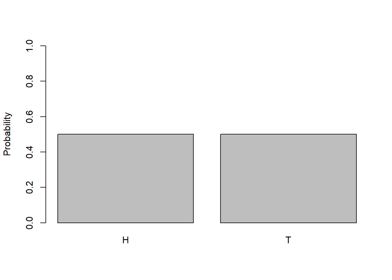
In this distribution we see that both outcomes have equal probabilities. And, importantly, this model also works for cases where \(p\) and therefore \(1-p\) are not both equal to 50%.
8.3.1 Expected Value and Variance
How would we find \(E[X]\) and \(Var[X]\)? I won’t derive this every time, but in this case its relatively simple.
For the expected value of \(X\) we only have two possible outcomes to deal with, so we have
\[E[X]= \sum X_i P_i = 1*p + 0*(1-p) = p\]
And really what this is saying, which is important, is that the average result will tend toward the probability of success. Maybe its obvious, but its nice that the math matches our intuition.
For the variance of \(X\), we first calculate \(E[X^2]\)
\[E[X^2]= \sum X_i P_i = 1^2*p + 0^2*(1-p) = p\]
and then use this to find Var[X] as:
\[Var[X] = E[X^2] - (E[X])^2 = p-p^2 = p(1-p)\] As we know, this tells us about how much spread exists around our results, and this will become more clear as we introduce more trials in the next section.
8.3.2 Parameterizing a Bernoulli Distribution
A Bernoulli random variable is parameterized simply by its mean \(\mu=p\), because once that’s known, the standard deviation is also: \(\sigma=\sqrt{p(1-p)}\)
So, for a fair coin, we’d have \(\mu = 0.5\) and \(\sigma = \sqrt{p(1-p)} = 0.5\) For a weighted coin where \(p=0.75\), we’d have \(\mu = 0.75\) and \(\sigma = \sqrt{0.75*0.25} = 0.433\).
Both the variance and standard deviation decrease slightly as \(p\) moves away from 0.5.
8.3.3 Simulation in R
If we wanted to simulate 100 Bernoulli trials with \(p=0.5\) (which is the default), in R we’d use:
You don’t observe the parameter here because it is the default.
If we wanted to simulate 1000 Bernoulli trials with probability of success \(p=0.2\), in R we’d use:
And now the parameter is evident.
8.3.4 Summary and Review
In this section we introduced a Bernoulli trial, which is a single trial of an event with a known probability of success, \(p\). We derived its expected value and variance, talked about how to parameterize the distribution and how to simulate from it.
For the most part, this is a building block for more detailed analysis, in particular the Binomial distribution, as we’ll see shortly.
8.3.5 Guided Practice
- What are the mean and standard deviation of a Bernoulli trial if \(p=0.48\)? What if \(p=0.1\)? Explain any differences you see. Which leads to more uncertainty?
- Simulate 100 trials of a fair coin toss and calculate the average and standard deviation. How does this compare to the expected value?
- Assume you are polling voters about an issue in the upcoming election and assume for your question \(p=0.333\). If you were to ask 100 people, what would the expected number of “yes” results be?
8.4 The Binomial Distribution
I suspect the discussion of a Bernoulli trial left you wanting more, in particular because of the constraint of only 1 trial. Let’s relax that constraint. We will now introduce the idea of the Binomial distribution which will allow us determine the probability of a certain/specific number of successes in many (\(n\)) trials.
The goals for this section include explaining what the Binomial distribution is and how its used. Here we’ll be looking at questions like: “if we toss a fair coin 20 times, what is the probability of seeing exactly 5 heads?” We know how to do this by hand, although it would be cumbersome, so here we’ll learn an easier way.
Specifically, the Binomial distribution is used to calculate the probability of a chosen number of success \(k\) in a fixed number of trials \(n\), assuming a probability of success on any given trial of \(p\), which we’ll write as \(P(X=k|n, p)\). Here, \(X\) is our random variable and \(n\) and \(p\) are parameters of our model.
In a moment we’re going to write down the analytical solution for the binomial distribution. But before we do that, let’s do an example by hand, just to remind ourselves.
8.4.1 How Many Successes?
For this section, let’s look at this question: “If we toss a weighted (unfair) coin three times, what is the probability of exactly two successes?” Here we
will define flipping a head as a success and because of the weighted coin, we will define \(p=0.6\).
Well first, what are the possible outcomes? Since each coin can be either H or T, there are \(2^3=8\) possible ordered outcomes:
| toss 1 | toss 2 | toss 3 |
|---|---|---|
| H | H | H |
| H | H | T |
| H | T | H |
| H | T | T |
| T | H | H |
| T | H | T |
| T | T | H |
| T | T | T |
Since this is NOT a fair coin, we need to be a little careful. What is the probability of any one row? In fact it depends on the row.
We know the individual probabilities of H and T, and since each coin flip is independent we can just multiply the probabilities. So, the probability of HHT is \((0.6)^2*(0.4)^1\), where the \((0.6)^2\) represents the probability of 2 successes and the \((0.4)^1\) represents the probability of 1 failure. And since there are 3 ways this can happen (HHT, HTH and THH), the probability of exactly two successes is \(3*(0.6)^2*(0.4)^1 = 0.432\).
(Of course I don’t need the exponent on the \(0.4\), however I’m using it to illustrate that we have exactly 1 failure.)
8.4.2 The Formal Binomial Distribution
Ok, so now that you understand how to calculate this by hand, I’m sure you can imagine that if \(n\) was much bigger than 3 it could become pretty tedious. Luckily there’s an easier way.
Formally we can write the binomial distribution as:
\[ P(X=k|n, p) = {n \choose k} p^k (1-p)^{(n-k)}\]
We read this as “the probability that our random variable \(X = k\) successes, given \(n\) trials and probability of success \(p\)”. Again, \(n\) and \(p\) are parameters of our distribution:
- \(n\) is the number of flips of a coin, or the number of people we poll.
- \(p\) is the probability of success on any given trial (one flip or one ask).
We’ve seen the choose() function \({n \choose k}\) before. To remind you, it calculates how many different ways can you choose \(k\) items from a set of \(n\) without worrying about the order. As a reminder:
\[{n \choose k} = \frac{n!}{k!(n-k!)}\]
So the first part of the Binomial distribution calculation accounts for the number of ways the desired outcome could occur, and the second part accounts for the probabilities of any particular outcome. In fact, this is just like what we did by hand, and the same approach we used in previous chapters.
Let’s plug in values from our above example to prove to ourselves it works. We had asked “If we toss a coin three times, what is the possibility of exactly two successes (again defining a head as a success)?”
\[\begin{eqnarray} P(X=2|n=3, p=0.6) & = & {3 \choose 2} 0.6^2 (1-0.6)^{(3-2)} \\ & = & 3 * 0.6^2 * 0.4^1 = 0.432 \end{eqnarray}\]
which happily gives the exact same calculation and result we did above!
A quick note about the notation. The pipe | character is the same as we used with conditional probability. We are determining the probability of a certain number of success “given” the parameter values.
But wait, didn’t you say this was going to be easier?!?! Hang tight.
8.4.3 Guided Practice
Let’s suppose we’re sampling from the general population about whether they like vanilla or chocolate better. And let’s suppose that 65% of the people prefer chocolate and 35% wrongly prefer vanilla.
If we draw 10 people at random, what is the probability that exactly 4 of those 10 prefer chocolate?
8.4.4 Answer
We could certainly attempt to do this by hand. But again, tedious…
Plugging this in to our formal definition above we set \(p= 0.65\) since we’re defining preferring chocolate as success. our total sample size is \(n=10\) and we’re looking for exactly \(k=4\) successes. Hence:
\[\begin{eqnarray} P(X=4|n=10, p=0.65) & = & {10 \choose 4} * 0.65^4 * 0.35^6 \\ & = & 210* 0.1785* 0.00184 = 0.0689 \end{eqnarray}\]
Or so there’s a 6.89% chance of finding that exactly four out of 10 people prefer chocolate.
8.4.5 Important Assumptions of the Binomial Model
Before going on, it’s important that we understand the assumptions or conditions that need to be true when using this model. These include:
- The trials are independent
- The probability of success for each trial is the same.
- The number of trials, \(n\) is fixed
- We can classified the outcome of each trial as a success or failure
8.4.6 Visualizing the Binomial Distribution and Calculating Probabilities
Now that we know how to calculate the probabilities of any given outcome, let’s visualize the distribution and think about calculating probabilities above or below a given value.
Imagine flipping a fair coin 6 times. We could see anywhere between 0 and 6 successes, right? Here’s a plot of the possible results, assuming we define seeing a head as success:
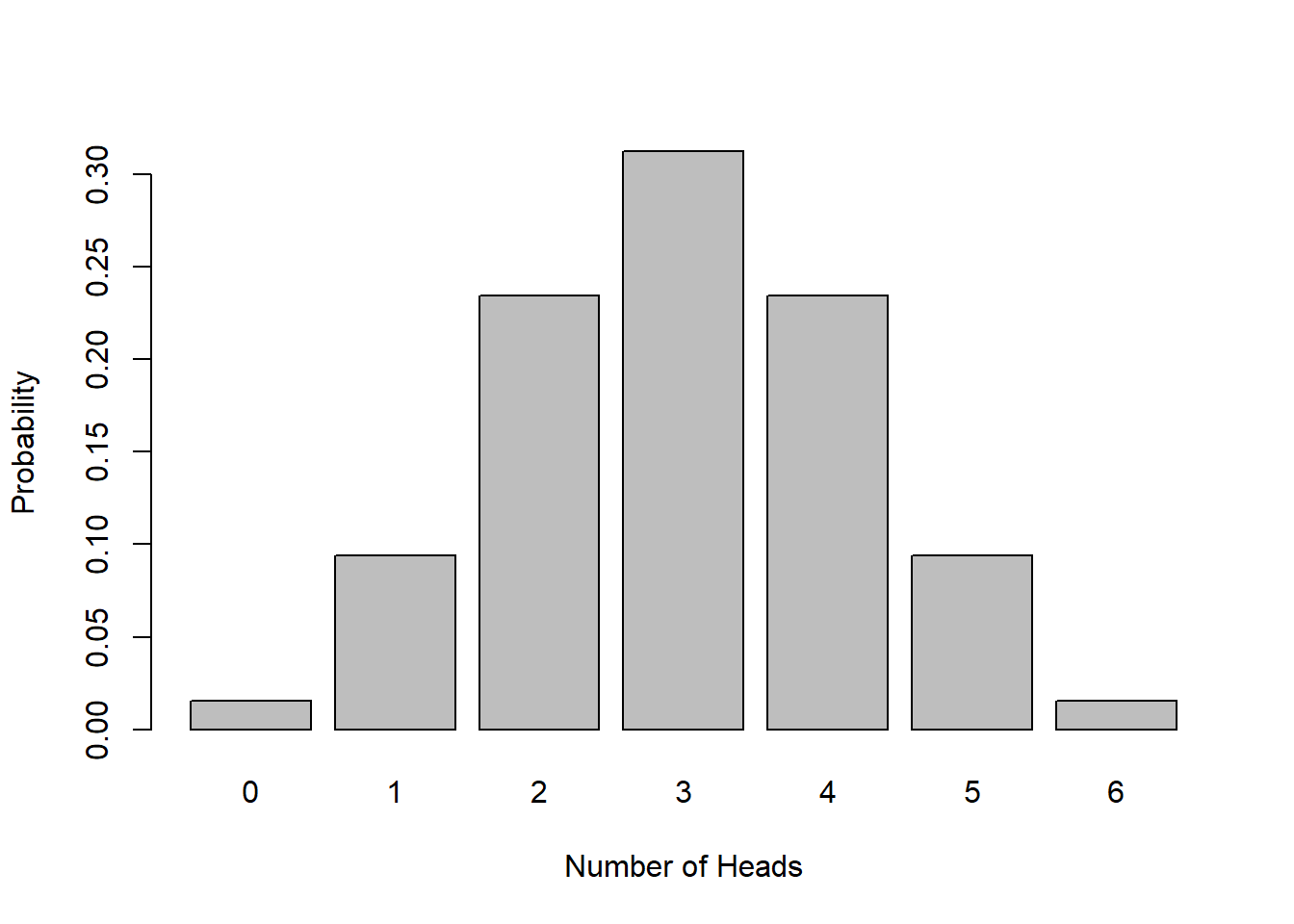
And here is a table of the specific probabilities of each outcome:
| \(k\) # of success | \(P(X=k)\) |
|---|---|
| 0 | 0.0156 |
| 1 | 0.0937 |
| 2 | 0.2344 |
| 3 | 0.3125 |
| 4 | 0.2344 |
| 5 | 0.0937 |
| 6 | 0.0156 |
What do you see? What do the heights of the bars add to? Why is it symmetric?
Based on this, how would you calculate the probability of seeing 4 or more successes, \(P(X\ge4)\)? As we previously discussed, we need to simply sum up the outcomes of interest here and/or ‘sum the area under the curve’. From this table, we calculate this to be: \[0.2344 + 0.0937 + 0.0156 = 0.3437\] or there’s a 34.4% percent chance.
You could use a similar approach to find \(P(X<1)\) or any other value.
8.4.7 Expected Value and Variance of the Binomial Model
What about the expected value and variance of the Binomial model?
I won’t derive these here, and instead just give the results. However, you should be able to derive these on your own do this using the approach described earlier.
For the mean (expected value) we have: \[\mu = np\]
Does this make sense? Think again about what expected value tells us. We know the number of trials \(n\), and we know the probability of success of any given trial \(p\), so what is \(\mu\) in this case? Hint: the expected number of successes.
For the variance we have: \[ \sigma^2 = np(1-p)\]
What does the variance tell us? Again it is an indication of the spread of the expected results.
Of importance here, note that both the mean and the variance depend on the value of \(n\). What does that mean? As \(n\) (the number of people we poll) increases, both the mean and variance will increase as well. You should also recognize that both of these are the Bernoulli results multiplied by \(n\).
For the previous example with \(p=0.5\) and \(n=6\), (i.e. flipping a fair coin 6 times), what are \(\mu\) and \(\sigma\)? We find \(\mu = 6*0.5 = 3\) meaning we would expect, on average, 3 successes. This is probably intuitive.
For variance, we’d find \(\sigma^2 = 6*0.5*(1-0.5) = 1.5\) and so the standard deviation is \(\sigma = 1.225\). To interpret this, think about how standard deviation relates to spread. And, think about where this would appear on the graph of the distribution.
8.4.8 The Binomial model in R
OK, I’m finally ready to answer the question about making this easier. R, as a statistical computing program, has built in functions to do this for us.
There are a few types of calculations we might want R to help us with. We’ll start with two: how to simulate data from a distribution and how to calculate the probability of a certain outcome.
8.4.9 Simulating data in R
First, we might want to simulate data from a binomial distribution. If you thought about this for a bit you might think we could use sample again as we’ve done previously. Possibly true, but there’s an easier way.
R has a function rbinom() which is a random generator for the binomial distribution.
Let’s go back to our ice cream example above. What we’re simulating is taking one sample of 10 people, asking type they prefer (chocolate or vanilla) and the recording the number of success. In R, we’d code this as:
## [1] 6The 1 indicates we’re only asking for 1 sample, the 10 is how many people we’re asking, and the p=0.6 gives the probability of success. R returns the number of people out of 10 who prefer chocolate in our random sample.
We could do more draws by increasing the 1 value and each of those samples would be independent, as if we were repeating the experiment by asking 10 different people.
8.4.10 Calculate the Probability of a Certain Outcome
The second thing we can easily do in R is estimate the probability of a specific outcome. This is the calculation we did by hand (above) and the R function to do this is dbinom, because it is the probability density. To estimate the probability of exactly four people who prefer chocolate, we’d code this as:
## [1] 0.0689098which matches our result above. Hopefully you agree this is much easier!
8.4.11 Guided Practice
- For this problem use a binomial distribution with probability of success of \(p=0.33\) and \(n=4\) trials. Do each of the following by hand and using the
dbinom()function in R to prove they match.
- What is the probability of seeing exactly 3 successes?
- What is the probability of seeing exactly 0 successes?
- What is the probability of seeing 1 or more successes?
- You are interested in sampling student’s preferences between Instagram and TikTok and believe that student’s prefer Tiktok 55% to 45%. You designate Tiktok a “success”, and you ask 8 random people.
- What is the probability that 6 or more people prefer TikTok?
- If you ask a group of friends, is the assumption about independence satisfied? Why or why not?
- What are the mean and variance for this situation?
8.4.12 Plotting a Binomial Distribution
From the previous guided practice we had:
You are interested in sampling student’s preferences between Instagram and TikTok and believe that student’s prefer Tiktok 55% to 45%. You designate Tiktok a “success”, and you ask 8 random people.
Let’s attempt to visualize this distribution.
The steps to plot a binomial distribution include:
- create the vector of possible outcomes (x-values)
- use the x values to create a vector of associated probabilities (y-values), which will be based on the given distribution
- for discrete random variables, use the
barplotfunction
- add the outcome labels and format the rest of the plot as desired
Steps 1 and 2 shown are below. For our probabilities (y-values) we use the dbinom() function where we pass it a vector of \(k\) values (our x vector), and it returns a vector of associated probabilities. This is a key step: dbinom() as with many R functions, will return a vector (list of values) if the input is a list of values.
It is not necessary to output the x and y values from this chunk, it is being done here only to illustrate the results.
## [1] 0 1 2 3 4 5 6 7 8## [1] 0.001681513 0.016441456 0.070332895 0.171924854 0.262662971 0.256826017
## [7] 0.156949232 0.054807668 0.008373394Just to check this, let’s calculate the sum of the y vector, which should add to 1 (since it’s a probability distribution!)
## [1] 1Now, we attempt to plot the results, and here we’ll use the barplot function to create the vertical bars representing probabilities. To assign the outcome labels, we use the names.arg parameter, and can simply assign it our outcomes x. Additionally here I’ve added parameters to set the x and y axis labels and plot title.
barplot(y, names.arg=x, xlab="# who prefer TikTok", ylab="Probability", main="Distribution of Tiktok vs. Instagram Preference", ylim=c(0,0.35))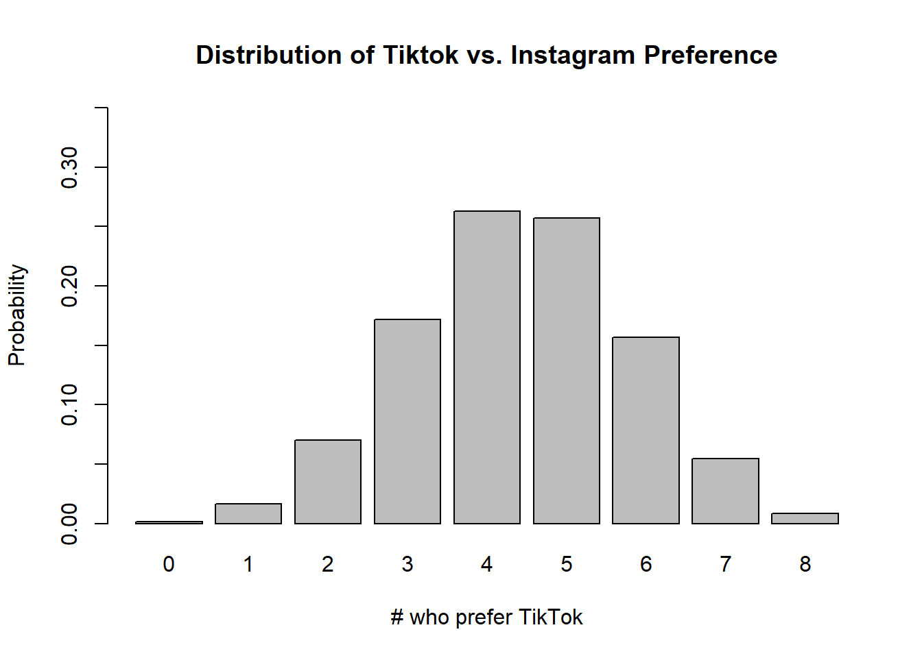
8.4.13 Are Binomial Distributions Always Symmetric?
No, binomial distributions are NOT always symmetric, it depends on values of \(p\). Our previous plot was slightly asymmetric.
Below is the Binomial Distribution for \(p=0.75\) and \(n=6\). Note in this case our mean is \(np= 4.5\).
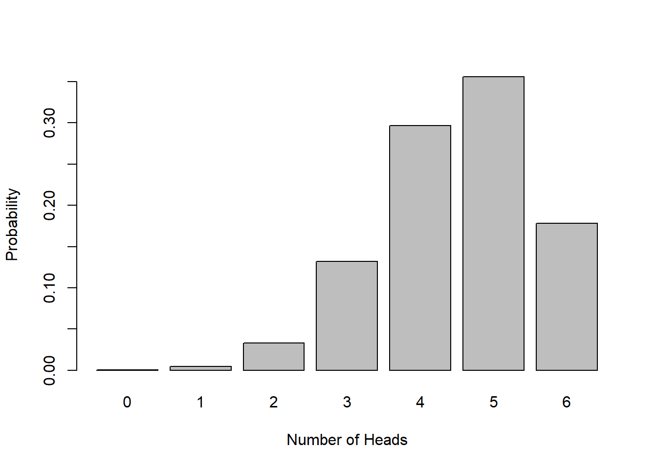
As \(p\) gets further away from \(p=0.5\), the more skewed the distribution will appear.
8.4.14 Summary and Review
In this section, we have learned:
- About the binomial distribution, when it’s used and the technical formulation
- About the parameters of the binomial distribution and its mean \(\mu = np\) and variance \(\sigma^2 = np(1-p)\)
- How to visualize the Binomial distribution (and btw, what happens as \(n\) gets large?)
- How to use R to both draw random samples from a Binomial distribution and to calculate probabilities.
8.5 Introducing Cumulative Probabilities
We previously discussed an example where we calculated the probability of seeing at least 4 or more successes when flipping a fair coin 6 times, and found the answer to be 0.34375. To do this, we calculated \(P(X=4) + P(X=5) + P(X=6)\), i.e. the probability of seeing exactly 4 success plus the probability of seeing exactly 5 success plus the probability of seeing exactly 6 success. As you could imagine, this could get tedious for larger numbers, and luckily it turns out there’s an easier way.
This type of calculation, particularly where we’re trying to determine the probability of seeing at least some specific result, or at most some other specific result, occurs a lot in statistics. So much so that we have a special type of distribution to help us work with these situations. These special distributions are known as cumulative distributions.
8.5.1 Cumulative Distribution
The cumulative distribution gives the probability that a random variable \(X\) will take a value less than or equal to some specified result, such as \(P(X\ge 4)\).
Let’s do a similar but slightly different problem. When flipping a fair coin 6 times, what is \(P(X\le 2)\) (the probability of 2 or less successes)?
As a reminder, here’s a quick table of results for each single outcome, i.e. \(P(X=i)\) and how to calculated them in R using dbinom(). This is also just our probability distribution for a Binomial(6, 0.5) model.
| num successes | \(P(X=i)\) | R function call |
|---|---|---|
| 0 | 0.015625 | dbinom(0, 6, 0.5) |
| 1 | 0.09375 | dbinom(1, 6, 0.5) |
| 2 | 0.234375 | dbinom(2, 6, 0.5) |
| 3 | 0.3125 | dbinom(3, 6, 0.5) |
| 4 | 0.234375 | dbinom(4, 6, 0.5) |
| 5 | 0.09375 | dbinom(5, 6, 0.5) |
| 6 | 0.015625 | dbinom(6, 6, 0.5) |
But what we want is to find find the the probability of seeing 0, 1 or 2 successes. To find this we’d add the first three rows to get 0.34375.
Formally, a cumulative distribution is the probability that a random variable \(X\) will take a value less than or equal to some specified result, \(P(X\le i)\).
Here is the table of cumulative probabilities for our situation of flipping a coin six times:
| num successes | \(P(X \le i)\) |
|---|---|
| 0 | 0.015625 |
| 1 | 0.109375 |
| 2 | 0.34375 |
| 3 | 0.65625 |
| 4 | 0.890625 |
| 5 | 0.984375 |
| 6 | 1 |
The cumulative probability of a 2 here means seeing 2 successes or less. The cumulative probability of a 0 here means seeing just 0 successes, and since there’s only one outcome here, the cumulative probability and the standard probability are the same. And the The cumulative probability of a 6 here means seeing a 6 or less, but since all outcomes are 6 or less, that last one must be 1 (i.e. 100%).
8.5.2 Visualizing the Cumulative Binomial Distribution
I think it’s worth showing the plot here.
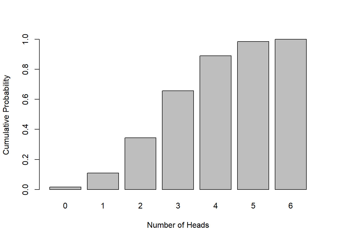
Cumulative probability plots will always have a similar shape, namely where it starts at with a y value equal to 0 and ends with a y value equal to 1, although of course the associated x values will change.
8.5.3 Calculating in Cumulative Probabilities in R
We’ve already seen how to calculate the probability of a single outcome occurring in R, using dbinom(). Here, we use a similar function, pbinom(). To use this function to calculate the probability of 3 or less successes we’d code this as:
## [1] 0.65625which seems to match the graph above. Again, this is the probability of seeing 0, 1, 2 or 3 successes. We could also say the probability of seeing at most 3 successes.
8.5.4 The Complement
But, what if we wanted the probability of at least four successes? Logically, we either see 3 or less successes OR we see 4 or more successes. One of those two events has to happen. So, if we can calculate the former, we can use our knowledge of complements to calculate the latter.
Hence, the probability of seeing at least 4 or more successes when flipping a fair coin 6 times is simply 1 - (the probability of seeing 3 or less successes). In R we can code this as
## [1] 0.34375which matches our above result!
We might write this as:
\[P(X\le k) + P(X>k) = 1\]
Or we might also write this as
\[P(X< k) + P(X\ge k) = 1\]
8.5.5 Be careful of your choice of \(k\)
In the R code above for determining the probability of 4 or more, we used a value of 3 as our parameter. Why? Because \(P(X\le 3) = P(x<4)\)
There are four ways we might ask this for a given \(p\), \(n\) and \(k\).
| calculation | R call |
|---|---|
| \(P(X\le k)\) | pbinom(k, n, p) |
| \(P(X> k)\) | 1-pbinom(k, n, p) |
| \(P(X< k)\) | pbinom(k-1, n, p) |
| \(P(X\ge k)\) | 1-pbinom(k-1, n, p) |
In particular this is an issue for discrete distributions (that we don’t have with continuous distributions).
8.5.6 The Cumulative Uniform Discrete Distribution
The idea of a cumulative distribution can be applied to any underlying distribution. Let’s go back to the discrete Uniform with min=1 and max=8.
What is the probability of \(P(X\le 3)\)?
8.5.7 Guided Practice
Back to our Tiktok vs Instagram example, where we assumed student’s prefer Tiktok 55% to 45%, we designated Tiktok a “success”, and asked 8 random people:
- What is the probability that 4 or less people prefer Tiktok?
- What is the probability that at least 5 people prefer TikTok?
- What is the probability that at most 5 people prefer TikTok?
- What is the probability that 6 or more people prefer TikTok?
8.5.8 Summary and Review
The brilliance of the cumulative distribution is that it really simplifies our life when we’re asking questions like “what is the probability of seeing at least 50% success?”
Each main distribution we’ll deal with has its own special version of the cumulative distribution.
We’ve seen how to use R to calculate a value from this distribution for the binomial distribution. And we’ve seen how to use the complement function (ok, really 1-x) to find the probabilities of seeing greater than a certain specified result.
8.6 Optional: Other Common Discrete Distributions
- Multinomial - I won’t talk about this, but imagine there were three (3) possible outcomes each with its own probability (that still sum to 1) Could you modify the above formal definition to account for this?
- Poisson - typically used to count the number of occurrences of a rare event. (In fact, the classic Poisson example is the data set of von Bortkiewicz (1898), for the chance of a Prussian cavalryman being killed by the kick of a horse.) Formally we write
\[P(X=k) = \frac{\lambda^k \exp^{-\lambda}}{k!}\] where \(\lambda\) is the mean of the distribution.
- Geometric - describes the number of trials until our first success, or more specifically, the probability that the first success we see is on the \(nth\) trial. Formally
\[P(X=n) = (1-p)^{n-1}p\]
with mean of \(\frac{1}{p}\)
8.7 Review and Summary
By the end of this chapter you should be able to:
- Define the discrete uniform distribution, a Bernoulli trial, and Binomial distribution and describe a situation where each might be applicable
- Define what is meant by a parameter of the distribution.
- List the parameters of the three above distributions and explain the impact of the parameter values on the distribution’s shape and therefore resulting probabilities
- Sketch (by hand or in R) the shape of each of these distributions
- Calculate the mean (\(\mu\)), variance (\(\sigma^2\)) and standard deviation (\(\sigma\)) for each of the above distributions
- Simulate random outcomes (using R) from each of the above distributions
- Calculate the probability density \(P(X=x)\) for each of the above distributions, both by hand and using the built-in R functions
- Explain what a cumulative distribution function is, i.e. \(P(X\le x)\), why it's important, how it’s used, and how to calculate it (in R or by hand) for each of the above distributions. Describe the end behavior of the cumulative distribution.
Here is a summary table of the main distributions we’ve studied:
| Distribution | Probability Density | Parameters | Mean | Variance |
|---|---|---|---|---|
| Discrete Uniform | \(P(X=i) = \frac{1}{b-a+1}\) | \(a, b\) | \(\frac{a+b}{2}\) | \(\frac{(b-a+1)^2-1}{12}\) |
| Bernoulli Trial | \(P(``success")=p\) | \(p\) | \(p\) | \(p(1-p)\) |
| Binomial | \(P(X=k|n, p) = {n \choose k} p^k (1-p)^{(n-k)}\) | \(p, n, k\) | \(np\) | \(np(1-p)\) |
8.8 Summary of R functions in this Chapter
| function | description |
|---|---|
barplot() |
function used to create plots of probability distributions |
rbinom() |
generate random data from a binomial distribution |
dbinom() |
calculate probability density for a binomial distribution |
pbinom() |
calculate cumulative probability for a binomial distribution |
8.9 Exercises
Exercise 8.1 If \(X\) is a random variable from a discrete uniform distribution with min: \(a=4\) and max: \(b=12\):
- How many possible outcomes are there?
- What is the probability of each outcome?
- What is the expected value and standard deviation of the distribution? (you can use the given formulas).
- What is \(P(X=6)\)?
- What is \(P(X\ge 6)\)?
Exercise 8.2 The barplot function in R can be used to create nice looking plots of discrete probability distributions. In this problem you will work through how to create one for a discrete uniform distribution.
For this problem, let \(X\) be a random variable that represents the roll of an 8 sided die.
- Create a vector that is 8 elements long with each value equal to 1/8. Hint: use the
rep()function and/or see the example in the notes above.
- Now plot your vector using the
barplot()function, passing your vector from part a as the only parameter. Also here add theylim=c(0,1)parameter to extend the range of your y-axis to range between 0 and 1.
- Your plot from part b does not have x axis labels. To fix this we will use the
names.argparameter. Addnames.arg=seq(1:8)as a parameter to the barplot() function. - Now add appropriate color, x-axis label (
xlab=" "), y-axis labels (ylab=" ") and title.
Exercise 8.3 Simulate 10000 random draws from a discrete uniform distribution with min: \(a=1\) and max: \(b=10\).
a. What are the mean and standard deviation of your sample?
b. Compute the expected mean and standard deviation using the formulas given above.
c. How close are your results between parts a and b? Explain any differences that you observe.
Exercise 8.4 How does \(p\) impact the mean and standard deviation of a Bernoulli trial?
- Imagine a Bernoulli trial with probability of success = 0.25. What are the expected value and standard deviation?
- Now imagine a Bernoulli trial with probability of success = 0.75. What are the expected value and standard deviation?
- Comment on any similarities or differences you see between parts a and b.
Exercise 8.5 According to a Pew Research poll (https://www.pewresearch.org/fact-tank/2018/12/10/social-media-outpaces-print-newspapers-in-the-u-s-as-a-news-source/) 36% of people 18-29 get their news from social media.
If we randomly ask 20 people in that age group about their primary news source:
- What are \(n\), \(k\) and \(p\) in this scenario?
- What is the probability that exactly 9 those people get their news from social media? Do this calculation both by hand and in R using
dbinom()to confirm the same results.
- On average, how many people would you expect of this group to say they get their news from social media?
- What is the probability that exactly 0 do? Explain why this answer makes sense.
- Create a plot (using
barplot) of the the entire distribution.
Exercise 8.6 Let’s suppose we’re sampling from the general population about whether they like vanilla or chocolate better. And let’s suppose that 65% of the people wrongly prefer chocolate and 35% prefer vanilla. You ask randomly poll 20 people about their preferred ice cream choice.
- Simulate 1 sample of 20 people from this binomial distribution. Do this a few times to confirm it works.
- Now simulate 50 samples of 20 people from this distribution. (Note that your result vector should have 50 elements).
- Calculate the mean of the simulated data. Then, compute the theoretical mean result, using the above equations for mean.
- Compare your answers to b and c.
- Now simulate taking many 20 person samples. Maybe take 100 then 1000 then ?? samples.
- Discuss what you observe about the mean, as “many” gets bigger.
Exercise 8.7 The probability of salmon going extinct in any one of a certain set of 5 watersheds within the next 10 years is estimated at 5%.
- What is the probability that none of the watersheds go extinct?
- What is the probability that two or less go extinct?
- What is the probability that two or more go extinct?
- What is the expected value of this distribution and what does it mean? Interpret its magnitude.
- Does it make sense to assume that these watersheds all act independently?
Exercise 8.8 You survey 20 potential voters about whether they think the environment or the economy was their highest concern, and let’s define success as them answering the environment with probability \(p=0.4\).
- What is the probability that exactly 11 of them say the environment? What are \(n\), \(k\) and \(p\) in this scenario? Solve this by hand and using R to confirm your results. (Hint: 20 choose 11 is 167960)
- What are the expected value and standard deviation of the results?
- What is the probability that 10 or less people cite the environment as their highest concern?
- What is the probability that more than 10 people do? (i.e. a majority)
Exercise 8.9 At this point in the 2019 season, the Seahawks had played 9 games and were 7-2, a winning percentage of 0.772. If we take this as the probability of them winning any game, and they had 7 games left,
- What is the probability that they would win at least 5 of the remaining games?
- How many of the remaining games would we expect the Seahawks to win?
- What is the probability that they would win at most 2 of the remaining games?
- Does it seem reasonable to assume that the probability of winning each remaining game is the same?
Exercise 8.10 Listen to this: https://www.npr.org/2019/10/30/774850885/what-stats-tell-us-about-how-much-being-the-home-team-matters-in-sports.
- Based on what you learned, what is the probability of the away team winning every game, assuming a 7 game series, and assuming the teams are otherwise evenly matched?
- What is the probability of the home team winning every game?
- If there have been 200 seven (7) game series (across a variety of sports and seasons), in how many of those would you expect to have the away team win every game, assuming the same probabilities?
Exercise 8.11 Since the year 2000, the S&P 500 (a stock market index) has had 13 years with positive returns and 5 years with negative returns. If we assume these data are representative:
- If we want to calculate the probability that at least 3 out of the next 5 years will be positive, what are k, n and p?
- What is the probability that at least 3 of the next 5 years will be positive?
- Do the assumptions of the Binomial model seem to hold in this case? Why or why not?
Exercise 8.12 During the MLS regular season, there were 117 penalty shots and of those 94 scored. In the Sounders vs. Real Salt Lake playoff game, the game went to a shootout to determine the winner. A shootout is where each team gets 5 penalty shoots and at the end, whoever scored the most, wins. Assuming the regular season probability applies, what is the probability that all 10 shots score?
- What is the probability that the Sounders scored at least 4 of their shots?
- What is the probability that the Sounders scored 3 or less of their shots?
- What is the probability that more than 8 shots are scored in total?
- Do you think the assumptions of independence and identical distribution hold?
- (Bonus) What is the probability that both teams score the same number?
Exercise 8.13 Recently, a nurse commented that when a patient calls the medical advice line claiming to have the flu, the chance that he or she truly has the flu (and not just a nasty cold) is only about 4%. Of the next 25 patients calling in claiming to have the flu, we are interested in how many actually have the flu.
- What is the random variable and what are its possible outcomes?
- What is the probability that at least four (4) of the next 25 patients actually have the flu?
- For every 25 patients that call in, how many do you expect to have the flu?
Exercise 8.14 For a Binomial distribution, with p=0.54 and n=12,
- What is the probability of seeing exactly 4 successes?
- What is the probability of 4 or less successes?
- What is the probability of 4 or more successes?
Exercise 8.15 For a Binomial distribution with p=0.33 and n=20, simulate 2500 random trials and store the result in a vector.
- What are the theoretical mean (expected value) and standard deviation of the distribution?
- What are the mean and standard deviation of simulated results?
- What is the theoertical probability of seeing at least 10 successes?
- What percent of your simulated results had at least 10 successes?
Exercise 8.16 If you take a sample of 18 people about whether they like the Star Wars (success) or Marvel (failure) franchise better, with an estimate of \(p=0.60\):
- What is the probability that exactly 9 of them will say they like Star Wars better? Write your answer in as “\(P(X\le x)=\)”…
- What is the probability that 9 or less of them will say they like Star Wars better?
- What is the probability that 12 or more of them will say they like Star Wars better?
Exercise 8.17 Given a Binomial distribution with \(n=21\) and \(p=0.41\), use R to determine:
- What is the \(P(X=8)\)?
- What is the \(P(X<=12)\)?
- What is the \(P(X>=10)\)?
- What is the \(P(X<5)\)?
- Simulate 1000 samples from this distribution and calculate the mean and variance. How do your simulated results compare to the theoretical values (you will need to calculate the theoretical values by hand)?
Exercise 8.18 Colleges typically admit more students than they have room for, given they know that not all applicants will accept. Assume that for a given university, 80% of the students who are offered admission, accept the offer. If the school has room for 800 incoming freshman, how many spots should they offer?
Exercise 8.19 A proposed COVID vaccine is reported to be 95% effective.
- If the vaccine is given to 100 people, all of whom are eventually exposed to the virus, what is the probability that more than 5 of them will get the virus?
- If you learned that 21 people got sick after taking the vaccine, would you be surprised? Why or why not? (Hint: think about z scores here!)
- In the same situation, assume that 8% of people given the vaccine experience serious side effects. What is the probability that more than 5 of the 100 experience serious side effects?
- If, for someone who has been given the vaccine, the probability of getting the virus and experiencing serious side effects are independent, what is the probability that both occur to that given individual?
Exercise 8.20 To get one’s drivers license, a person must first pass their theory/written test and then pass their driving/practice test. Assume we are told that 80% of teenagers pass the written test, and of those who pass the written test, 60% pass the driving/practice test.
- What is the probability that an individual chosen at random passes both the written and practice/driving test? Use probability notation to explain your answer.
- If 150 teenagers attempt to get their license, what are the expected value and standard deviation of the number of teens who pass both?
- Use R to simulate the probability distribution. Justify the number of simulations you use. Create a well formatted plot of your simulation results. Describe the shape of your simulated results.
- Based on your simulation, what is the probability that between 65 and 85 (inclusive) of the 150 teens who attempt to get their license pass both tests? Show all R code.
- If you were told that only 54 teenagers out of 150 passed both their driving and written tests, would you be surprised or not? Why? Be as quantitative as possible.
Exercise 8.21 “If I want to drive from my home on Mercer Island to the Eastside Prep in Kirkland, I have two perfectly good roads to follow: take I-405 or Bellevue Way. Assume the drivers of 200 cars independently and randomly make their choice between these two roads with a 50 percent probability of choosing a given road. Also assume that there are no other cars on the road.
- What is the probability I pick the more crowded road?
- What is the probability that exactly 100 cars pick each road?
- What is the expected value of how many more of the 200 cars end up on the more crowded road?”
Source: https://www.quantamagazine.org/solution-the-road-less-traveled-20150925/
Exercise 8.22 Above I stated that \(E[X] = \frac{a+b}{2}\) for a discrete uniform distribution with \(a\) as the minimum and \(b\) as the maximum. Prove this is true.
Hints:
- Based on \(a\) and \(b\) how many outcomes are there?
- What is the probability of any outcome?
- Can you write the \(E[X]\) as a series in terms of (a) and (b)?
- Now, what is the sum of \(a ... b\)? You should be able to write this in terms of \(a\) and \(b\). It may be easiest to consider the cases where there are an odd or even number of elements separately.
- Combine (d) and (b) to prove the result.
Exercise 8.23 We can use the Poisson distribution to model the number of soccer goals scored in a game. Assume \(\lambda=2.5\) is the average number of goals scored in a game.
- Use the
dpois()function to calculate the probability of scoring 0, 1, 2, 3 and 4 goals.
- What is the sum of the probabilities from part a? Explain what you see.
- Create a plot of the distribution.
Exercise 8.24 The Geometric distribution can model the number of failures (or attempts) until the first success. Assume \(p=0.25\) is the probability of success.
- Use the
dgeom()function to calculate the probability that the first success occurs on the 2nd, 3rd, 4th or 5th trials.
- What is the sum of the probabilities from part a? Explain what you see.
- Create a plot of the distribution.