Chapter 10 The Normal Approximation and CLT
10.1 Overview
Now that we’ve examined the Normal Distribution, we’re ready to answer a question that was inaccessible before. What’s the likely distribution of results if we play “our game” many times?
We previously talked about what the expected value and variance of one turn of the game, but what if we play, say 100 times? What are the expected value and variance of our overall winnings? And similarly, we previously used the binomial distribution to ask \(P(X/n>0.5)\) (i.e. did our ballot measure or candidate win?), but what if \(n\) is really large, say 1,000,000? Those choose calculations can get pretty complicated.
In this chapter we’ll discuss how we can approximate these results using a Normal distribution, and how we can parameterize that Normal. We’ll also define and discuss the “Central Limit Theorem” which is the groundwork that allows us to make this approximation.
10.1.1 Learning Objectives
After this chapter, you should be able to:
- Describe what the Central Limit Theorem generally says
- Calculate the normal distribution of winnings and losses to our previous ‘games’, (as opposed to simply its mean and variance)
- Use your knowledge of the normal distribution to calculate associated probabilities of winning or losing certain amounts
- Understand that for large \(n\), a binomial distribution approximates a Normal distribution, and calculate the parameters of a Normal distribution that approximate the Binomial distribution
10.1.2 The Distribution of Sums
Let’s suppose we had a non-standard distribution, as shown below. Maybe this is an unfair (really unfair!), six sided die. The outcomes are still 1 through 6, and the total probability is still one, but here the probabilities of each outcome are NOT equal:
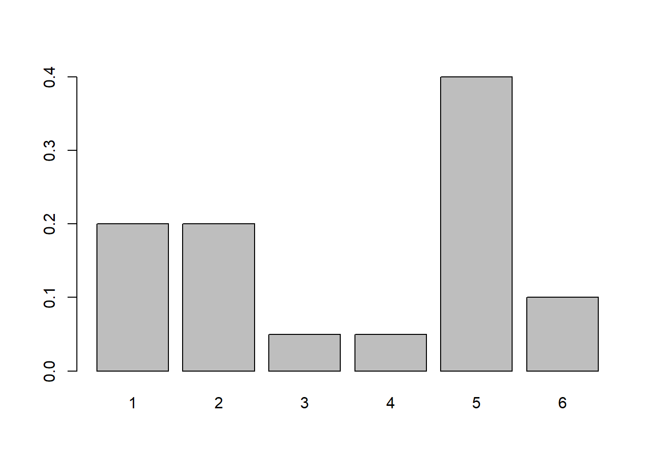
You could all calculate the mean and variance of this distribution using what we previously learned about discrete random variables.
If we did this, we would find \[E[X] = \sum X_ip_i = 1*0.2+ 2*0.2+3*0.05+ 4*0.05 + 5*0.4 + 6*0.1 = 3.55\] and \[Var[X] = E[X^2]-(E[X])^2 = 15.85 - 12.60 = 3.25\]
Instead here, I want to think about is the distribution of the sum of \(n\) rolls, i.e. if we played this game many times, what would the distribution (including mean and variance) of our winnings look like?
How might we calculate this? If we were doing just \(n= 2\) rolls, we could create a 6x6 table and figure out the probabilities of each sum. For anything more than that, it’s much easier (although a little less precise) to simulate these.
Here is the code and histogram of the sum of 2 rolls from 25000 simulations of this unfair distribution:
# set the number of times to run the simulation, pick a big number to reduce the variability
s <- 25000

# create a vector to store the results
rslt <- vector("numeric", s)

# main for loop, run through each simulation, draw two values and then add them together
for (i in 1:s) {
  rslt[i] <- sum(sample(x, 2, prob=myd, replace=T))
}

# plot out the histogram of results
hist(rslt, freq=F, breaks=13, main="sum of 2 rolls")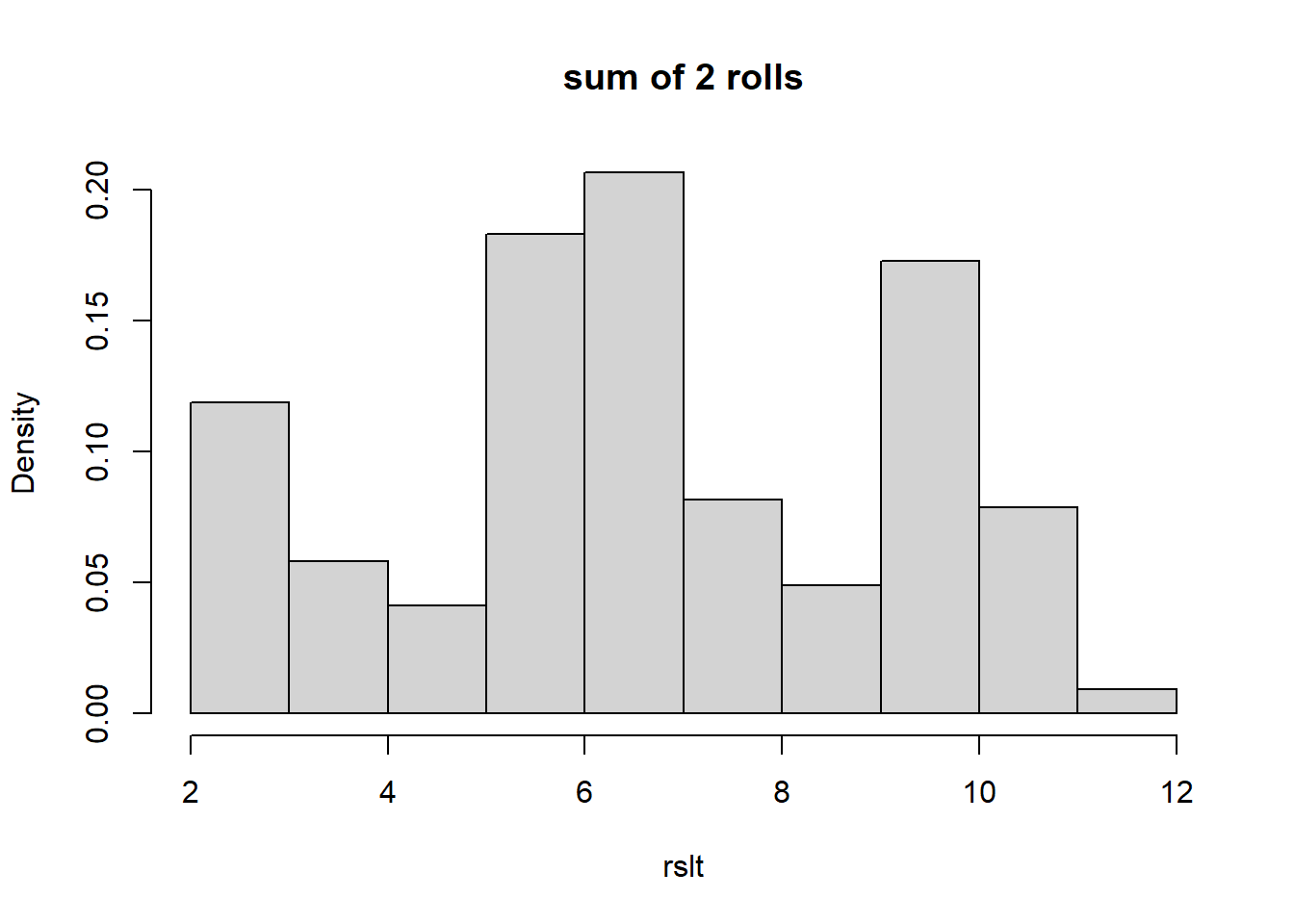
What do you notice? The possible outcomes range between 2 and 12. Probably not unsurprisingly, it has somewhat of an irregular shape, because of our underlying distribution.
Now, here is the sum of 5 rolls:
# set the number of times to run the simulation
s <- 25000

# create a vector to store the results
rslt <- vector("numeric", s)

# main for loop, run through each simulation, draw two values and then add them together
for (i in 1:s) {
  rslt[i] <- sum(sample(x, 5, prob=myd, replace=T))
}

# plot out the histogram of results
hist(rslt, freq=F, breaks=13, main="sum of 5 rolls")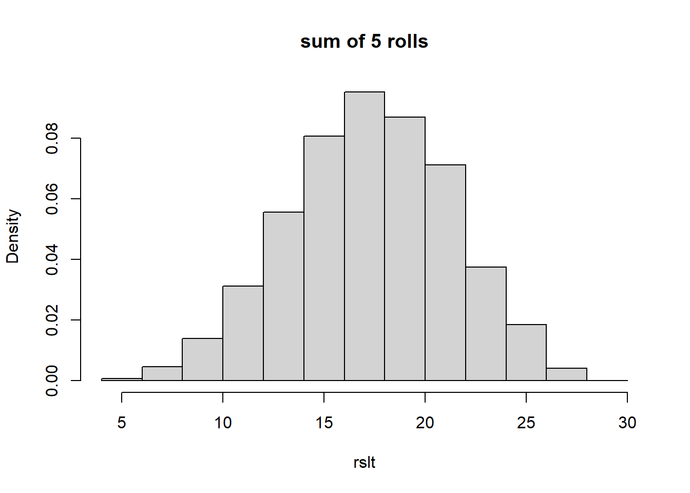
Now what do you notice? Particularly about the shape of the distribution. Does it remind you of anything?
Hopefully what you see is that even if we start with something pretty “ugly”, after we take the sum of random results from that original distribution, the result begins to look Normal, and it doesn’t even take many turns for that to happen. We see it above in simply 5 turns. In a nutshell, that’s what the Central Limit Theorem (CLT) says.
And, even better, if we know the mean and standard deviation of the underlying distribution, using the CLT we can parameterize the resulting normal approximation (distribution) pretty easily, which I’ll show shortly.
10.2 The Central Limit Theorem
What the Central Limit Theorem says is that sums (or averages) of random variables taken from “well behaved” distributions tend to be Normal as \(n\) (the number of samples or trials) grows large.
Here “well behaved” basically means that the underlying distribution has a finite mean and variance. So in the unfair die example above, or any of the games we’ve played, or even the Binomial distribution are all “well behaved” based on this definition.
More importantly, the CLT also says that if we start with a random variable \(X\) where we know its mean \(\mu_X\) and variance \(\sigma^2_X\), and if then we let \(Y\) be the sum of \(n\) IID turns of \(X\) (remember that IID means independently and identically distributed), then we can approximate the distribution of \(Y\) as:
\[Y\sim N(n\mu_X, \sqrt n \sigma_x)\]
So, if we’re calculating the sum (or average) of many turns or trials of a game or experiment where we at least know the underlying distribution’s (i.e. one trial’s) mean and variance, then we can represent this new random variable as having a Normal distribution.
Note this is true regardless of the underlying distribution (shape) of \(X\).
I won’t go through the details of the proof, but I may occasionally say “I’m appealing to the CLT here”.
And you should recognize that since average values are basically sums, the CLT applies to distributions of averages as well.
10.2.1 CLT and our Ugly Distribution
Let’s take the distribution from above and calculate the distribution of the sum of \(n=25\) rolls. Remember \(\mu_X = 3.55\) and \(\sigma_X = \sqrt{3.25} = 1.802\).
Using the definition of the CLT from above we have \(Y\sim N(25*3.55, 5*1.802)\) or \(Y\sim N(88.75, 9.01)\).
To show this is correct, let’s simulate the sum of 25 turns, and then overlay the distribution as predicted by the CLT.
# set the number of times to run the simulation
s <- 25000

# create a vector to store the results
rslt <- vector("numeric", s)

# main for loop, run through each simulation, draw two values and then add them together
for (i in 1:s) {
  rslt[i] <- sum(sample(x, 25, prob=myd, replace=T))
}

# plot out the histogram of results
hist(rslt, freq=F, breaks=13, main="sum of 25 rolls")

x <- seq(from=60, to=120, b=0.1)
y <- dnorm(x, 88.75, 9.01)
lines(x,y, col="red")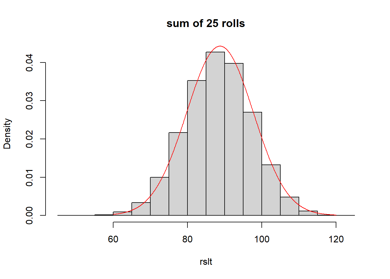
The normal curve shown in red, which was parameterized based on the CLT, fits the simulated distribution quite well.
10.3 Many Turns of our Game
A few weeks back when we introduced the long form to finding \(E[X]\) and \(Var[X]\) for discrete random variables, as our example, we played some games and could estimate the probability of winning any given roll. That left us a little wanting, though…
Here was one of the games we played:
It costs you $15 to play. You get to roll 2 dice. If the sum is 2, 3 or 12, you win $100. If the sum is 7 or 11, you get your money back. If any other sum (4, 5, 6, 8, 9, or 10) you win nothing and lose your $15. Would you play? And how would you decide?
We found \(E[X] = -0.556\) and \(Var[X] = 952.47\) (or equivalently a standard deviation of \(\sigma =30.86\)).
What if we wanted to understand the distribution of winnings after playing for an hours, say \(n=100\) turns?
Let’s apply the CLT formula: \[Y\sim N(n\mu_x, \sqrt n \sigma_x)\]
We will use \(n=100\), \(\mu_x = -0.556\) and \(\sigma_x = 30.86\) where the subscript \(_x\) refers to that random variable.
If \(Y\) is new the random variable representing the sum after 100 games, then \(\mu_Y = 100*-0.556 = -55.6\) and \(\sigma_Y = \sqrt{100}*30.86 = 308.6\). From this, we can write the distribution of \(Y\) as \(Y\sim N(-55.6, 308.6)\).
The mean here (\(\mu_Y = -55.6\)) should be somewhat intuitive. If we expect to lose -$0.556 per turn, and if we play 100 games/turns, then we’d “expect” to lose -$55.6 (on average) after 100 games. For the variance, it turns out we also multiply that by 100, and so the standard deviation increases by an order of 10 (the square root of 100).
10.3.1 Using the CLT
Now, because the CLT gives us a Normal distribution, we can use all of the tools we learned last chapter. For example:
- What is the probability that our winnings would be greater than 0?
We can use our parameterized normal distribution to find this as:
## [1] 0.4285101Or so there’s a 43% chance we would be above $0 after playing the game 100 times. Sort of surprising, right?
- What is the likely 95% range on our winnings?
Similar to above, we use the parameterized normal to find the boundaries of this range as:
## [1] -660.4449## [1] 549.2449So the 95% likely range on our winnings (in $) is within the interval between {-660.44, 549.24}.
10.3.2 Summary of using the Normal Approximation
The steps to using the CLT to find a normal approximation are to:
- Calculate the expected value (\(\mu_X\)) and variance (\(\sigma^2_X\)) of any single turn of the game (we did this previously)
- Let \(Y\) be the random variable that represents the sum after a certain number of turns, \(n\)
- Parameterize our new Normal distribution as \(Y\sim N(n\mu_X, \sqrt n\sigma_X)\) (and note we’re using the standard deviation here, so take the square root of the variance.)
- Use the appropriate R functions to calculate the probabilities or quantiles of interest using the distribution of \(Y\)
10.3.3 Guided Practice
Imagine a game with \(\mu_x = 1\) and \(\sigma_x = 25\). If we play the game \(n=25\) times, what is the probability that we’ll end up with at least $10? What is the likely 90% range on our winnings?
In the above example with \(\mu_x = -0.556\) and \(\sigma_x = 308.6\), what happens as to the probability of winning money as \(n\) gets larger? Calculate this for 200, 500 and 1000 turns and comment. Does the probability of winning money increase or decrease as \(n\) goes up?
10.4 Using the Central Limit Theorem on the Binomial Distribution
Caveat: It used to be that before computers were so powerful and accessible that the Normal approximation to the binomial distribution was critical to solve for large \(n\). How would you calculate choose for \(n=100\) or more by hand? Nowadays, R can easily do it even for values as large as \(n=20000000\).
As you’ll remember, the Binomial distribution is the sum of \(n\) independent Bernoulli trials. Each Bernoulli trial has mean \(\mu_x = p\) and variance \(\sigma^2_x = p(1-p)\) So, we can apply our Normal approximation above to estimate the binomial distribution as \[Y\sim N(np, \sqrt{np(1-p)})\]
This approximation replaces the Binomial distribution as previously discussed.
(NOTE: since I’m using variance here, the normal approximation variance is \(np(1-p)\) and so the normal approximation standard deviation is \(\sqrt{np(1-p)}\))
10.4.1 An Example of the Normal Approximation to the Binomial
Let’s imagine we’re asking people what they thought about Trump’s impeachment during early 2020. According to the website FiveThirtyEight.com, about 47.7% of people supported impeaching Trump.
If we had asked 1000 people, what’s the probability that at least 501 would have supported it?
We could find the exact answer using the binomial distribution as \(P(X \ge 501|n=1000, p=0.477)\) and as a reminder, in R we would calculate this as:
## [1] 0.06049181and we see there is an approximately 6.05% chance of greater than 50% of our sample supporting impeachment.
Now let’s use our normal approximation to compare. Based on above, for a single Bernoulli trial, we can write \(\mu_x = 0.477\) and variance \(\sigma^2_x = 0.477(1-0.477)= 0.2495\). If we let \(Y\) be the random variable that is the sum of IID Bernoulli trials, then for \(n=1000\), we find \(\mu_y = 1000*0.477 = 477\) and \(\sigma_y = \sqrt{1000*0.2495} = 15.80\). Thus, our Normal approximation to the binomial distribution is \(Y\sim N(477, 15.80)\).
Here is the plot of the binomial distribution (histogram) and normal approximation (in red) showing how the approximation fits:
y <- rbinom(5000, 1000, 0.477)
hist(y, freq=F, breaks=20, xlab="Number of successes", main="Binomial (n=1000, p=0.477)")

#x <- seq(from=430, to=535, by=2)
#y <- dbinom(x, 1000, 0.477)
#barplot(y, names.arg = x)

x2 <- seq(from=430, to=535, by=0.5)
y2 <- dnorm(x2, 477, 15.8)
lines(x2,y2,type="l", col="red")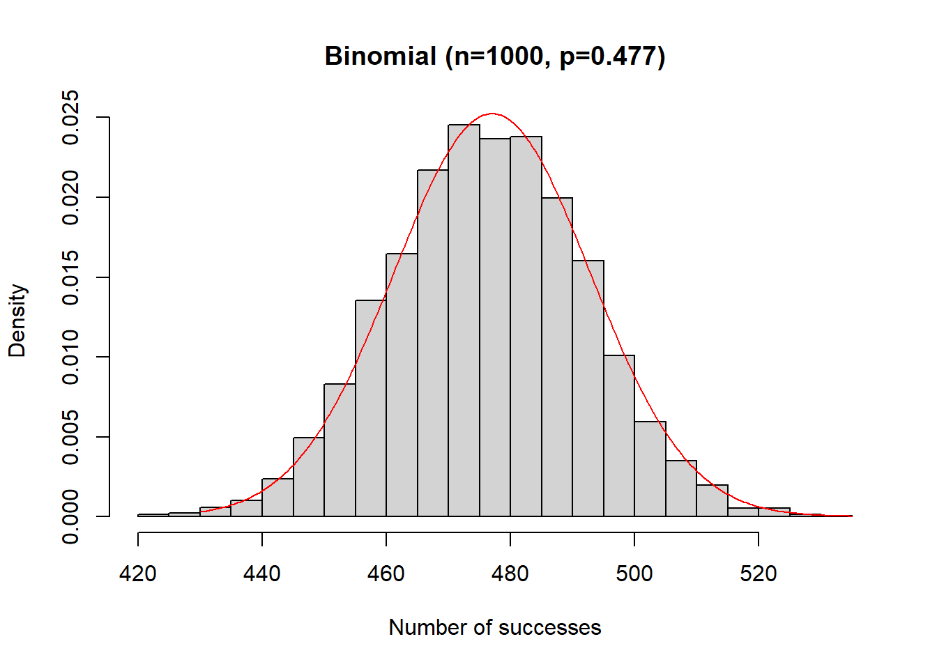
Now, let’s ask the same question as above, namely what is \(P(Y \ge 501)\), but based on our approximation? In R we would calculate this as:
## [1] 0.05574721Which says there’s approximately a 5.57% chance of seeing at least 501 people (\(\ge\) 50% of our sample) in support.
What we see is that the approximation is close, within 0.5%, which is reasonably close. This would get even better as \(n\) gets larger.
In summary, we can approximate a binomial distribution with parameters \(n\) and \(p\) using \[X\sim N\left(np, \sqrt{ np(1-p)}\right)\]
and then, once we have our Normal distribution, we can again use all of our normal functions to find probabilities and quantiles, etc. File this away as one of those things you should know exists.
10.4.2 Guided Practice
If you poll 150 people with an expected probability of success of \(p=0.45\):
- Using the Binomial distribution, what is the probability of seeing at least 120 successes? (Hint: use
pbinom()) - What are the mean and standard deviation of the approximate Normal distribution? Write down the short-hand for the approximate Normal distribution.
- Using the approximate Normal distribution, what is the probability of seeing a 80% success rate? (Hint: use
pnorm()) - How do the answers from the Binomial distribution and Normal approximation compare?
- Recreate the above histogram of the Binomial distribution using data simulated from
rbinom, and overlay the Normal approximation.
10.5 Simulating the Central Limit Theorem
As a last section to this chapter, we’ll demonstrate via simulation how well the CLT works.
Imagine the following game:
It costs you $1 to play. You roll two 6-sided dice and sum the results. If the roll is a 2, 3, or 12 you get your $1 back and win an extra $5. If you roll a 5, 9, or 11 you `draw’ and simply get your $1 back. Otherwise, you lose your original bet.
For this game we can calculate the mean as:
## [1] -0.05555556And similarly the standard deviation as:
## [1] 1.840055Based on the CLT, if we played this game 100 times, we’d expect the sum of our winnings to be distributed as \(Y \sim N(-5.56, 18.4)\)
Now, let’s use use R to simulate this game, and run many trials, then show that the CLT approximation is pretty good.
- Download
game_sim.Rfrom the labs folder on Canvas, source it. - Inspect the
one.roll()function and then callone.roll(T)a handful a times by typing it in the console. What do you notice. Does it recreate our game accurately? - Now execute the
many.trials()function. This should take about 30 seconds to run and will (i) create a histogram of the results from 10000 times of playing the game 100 turns, and (ii) return the descriptive statistics for the results of 10,000 simulations of 100 turns.
- How do your mean and standard deviation compare to the analytical result above?
10.6 Summary of Results
The following table shows how to parameterize the normal approximation for both the general case as well as the binomial model.
| Distribution | mean | variance | Normal Approximation |
|---|---|---|---|
| General | \(\mu_x\) | \(\sigma^2_x\) | \(Y \sim N(n\mu_x, \sqrt{n}\sigma_x)\) |
| Binomial | \(p\) | \(p(1-p)\) | \(Y\sim N(np, \sqrt{np(1-p)})\) |
and note that although we derived the binomial approximation using the Bernoulli results, the mean and variance we use within the approximation are simply the mean and variance of the binomial distribution itself.
10.6.1 Review of Learning Objectives
After this chapter, you should be able to:
- Describe what the Central Limit Theorem generally says
- Calculate the normal distribution of winnings and losses to our previous ‘games’, (as opposed to simply its mean and variance)
- Use your knowledge of the normal distribution to calculate associated probabilities of winning or losing certain amounts
- Understand that for large \(n\), a binomial distribution approximates a Normal distribution, and calculate the parameters of a Normal distribution that approximate the Binomial distribution
10.7 Exercises
Exercise 10.1 Assume, for a given game, that for each turn \(E[X] = 0.25\) and \(Var[X] = 1.75\).
- What is the distribution of your sum after 20 turns? Write this as \(Y\sim N(\mu, \sigma)\) where you calculate the appropriate values of \(\mu\) and \(\sigma\).
- What is the probability that after 20 turns you would win at least $10?
- What is the probability that after 20 turns you would lose no more than -$5?
- What is the likely 95% range on your winnings after 20 turns?
Exercise 10.2 Explain what the Central Limit Theorem says. Why does it apply to both sums and averages?
Exercise 10.3 Imagine you were taking 50 draws from a discrete uniform distribution with \(a=-3\) and \(b=4\).
- What is distribution of your sum?
- What is the probability your sum is greater than 10?
Exercise 10.4 In 2018, you took a sample of 250 people from a much larger population, asking about their support of a carbon tax in WA state, with an estimated probability of success, p=0.62.
- Assuming a Normal approximation to the Binomial distribution, what are the values of the mean and standard deviation?
- Given your sample size, how many people would you expect to show support for the initiative? Relate your answer to part (a).
- What is an approximate Normal distribution for your sample?
- Based on part c, what is the probability that at least 200 people indicated support for the carbon tax?
- What values are boundaries of the 90% most likely interval for the number of people who indicated support?
Exercise 10.5 In thinking about games of chance more generally:
- If you’re the casino, you want a negative expected value for the player. Explain why that’s true.
- Is it better for the casino to have a larger or smaller standard deviation on game results? When answering this, consider both their profits and what may entice players to remain at the table. Use numeric examples to support your arguement.
Exercise 10.6 For a given game, you calculate that \(E[X] = \$0.05\) and \(Var[X] = 2.33\). If you play the game 100 times:
- Explain what the value of \(Y\) is in this case. Why is it a random variable?
- Determine the parameters you would use within an approximate Normal distribution. Write down the short-hand for this approximate Normal distribution.
- What would your expected result be after 100 turns?
- Find the probability that after 100 turns you would win at least $10?
- What is the middle 90% range of results that you would see after playing 100 times? Write this as an interval.
Exercise 10.7 Imagine a game where you roll a single 10 sided die. You bet $2 and if the value is 1, 4 or 9, you square your bet! So, if you bet $2, if you win $4 plus get your original $2 back. Otherwise you lose your $2 bet.
- What are the expected value and variance of this game?
- If you were to play this game 20 times, what are the parameters of the Normal distribution to describe your total winnings or loses?
- If you were to play this game 20 times, what is the probability that you end “in the black”, meaning that your total winnings are greater than $0?
- If you were to play this game 20 times, what are the boundaries on the 95% likely range on your winnings or loses?
Exercise 10.8 Simulate the above game (\(E[X] = 0.25\) and \(Var[X] = 1.75\)) for many turns, keeping track of your total winnings. Create a plot of the winnings as a function of the turn number (x-axis). Describe the plot that you see. Where do the \(E[X]\) and \(Var[X]\) show up on this plot?
Exercise 10.9 In Lecture, I simulated the Binomial distribution and showed as \(n\) gets large, the distribution tends to Normal. Recreate this simulation, but now with different values of \(n\) and \(p\) and show that as the number of samples increases, the shape of the distribution looks more and more Normal. Choose a value of \(p\) that is not equal to 0.5 so you can prove to yourself that the Normal approximation doesn’t need a symmetric distribution as a starting point. Choose something extreme such as \(p= 0.25\) or \(p=0.75\). Include at least 3 histograms with different numbers of samples to show the evolution of the shape of the distribution.
Exercise 10.10 In 2018, you took a sample of 250 people from a much larger population, asking about their support of a carbon tax in WA state, with an estimated probability of success, p=0.62.
- Assuming a Normal approximation to the Binomial distribution, what are the values of the mean and standard deviation?
- Based on part a, and assuming a Normal approximation, what is the probability that at least 200 people indicated support for the carbon tax?
- What values are boundaries of the 90% most likely interval for the number of people who indicated support?