Chapter 1 Introduction to Probability Statistics
In this chapter, we’re going to introduce and discuss some of the concepts of probability and statistics that we’ll be covering this year, as well as introduce how and why R will be of such help to us.
1.1 The Lady Who Tasted Tea
Imagine you have a friend who drinks a lot of Starbucks coffee, and she claims she can distinguish whether milk is added before coffee or coffee is added first, i.e. before milk.
Do you believe her? How might you run an experiment to evaluate this? Think about specifics of your experiment.
1.1.1 Learning Objectives
- This is meant to act as an overview of the course. In this section we’ll be discussing probability and sampling, distributions, and hypothesis testing
- We’ll also see how useful R can be and why it’s our platform for the course
1.1.2 Following along in R
I’d suggest you follow along by opening R Studio and creating a new R Markdown file. (File -> New File -> R Markdown…). Add a meaningful title and then press OK. And DELETE everything after line 7. Those lines are not necessary and will add garbage to your final output.
Every time there is code to execute, you should add a new code chunk. The easiest way to do this is to either:
- Type: CTLR-ALT-I, or
- Insert -> R (just below the main ribbon)
1.2 Do You Believe Her?
Back to our friend… do we believe her? How would know?
1.2.1 Opportunity for Student Discussion
Some questions:
- Could we setup an experiment to test this?
- How much evidence would you need to believe (or disbelieve) her? For example, assuming 10 trials (guesses), how many out of 10 would she need to get right for you to believe her?
- In designing an experiment, how many of the trials should be coffee-milk vs. milk-coffee and in what order would you present them?
When I use the word trial, I mean one individual test where our friend is given a mixed cup of coffee and asked to tell us which order the coffee and milk were added. She will either get it right (“success”) or wrong (“failure”).
1.2.2 Ok, so Let’s Run the Experiment (sort of)!
In small groups of 2 or 3, choose one person be the experimenter and one be the coffee drinker.
- The experimenter will randomly select a list of 10 C (coffee first) and M (milk first), 5 each. For example, maybe the experimenter selected: MMCCMCMCCM. Keep this list hidden from the coffee drinker.
- Then in order, the coffee drinker will guess which type of drink is next.
- The experimenter should record how many (out of 10) the coffee drinker guesses correctly.
Then switch roles and repeat.
1.2.3 How Did We Do?
Tell me the number of successes each guesser had (out of 10)! I’ll fill in the R code and then we’ll plot the results.
successes <- c(4, 8, 5, 7, 7, 5, 6, 4, 6, 9, 5, 6)
barplot(table(successes), ylab="# of times", xlab="# of Successes")
So, this distribution shows us how many times (on the \(y\)-axis) we saw each number of successes (on the \(x\)-axis) out of 10.
1.2.4 Simulation in R
We can also let R do this for us. The following code simulates a single experiment with 10 trials where the probability of success for each trial is \(p=0.5\). (If you run this code you will likely get a different result - because of the random number generator!)
## [1] 5The rbinom() function here simulates a random number of successes for our experiment, with \(n=10\) and \(p=0.5\). (Technically we’re using a Binomial distribution here, but more on that later.)
Press the green “play” button to rerun this code and you should see your results change.
This next chunk of code runs 1000 different experiments! And then displays the results. (Either type it as is, or simply copy it over into a new R chunk.)
rslt <- rbinom(1000, 10, 0.5)   ## store the results in a variable called 'rslt'
barplot(table(rslt), ylab="# of times", xlab="# of Successes")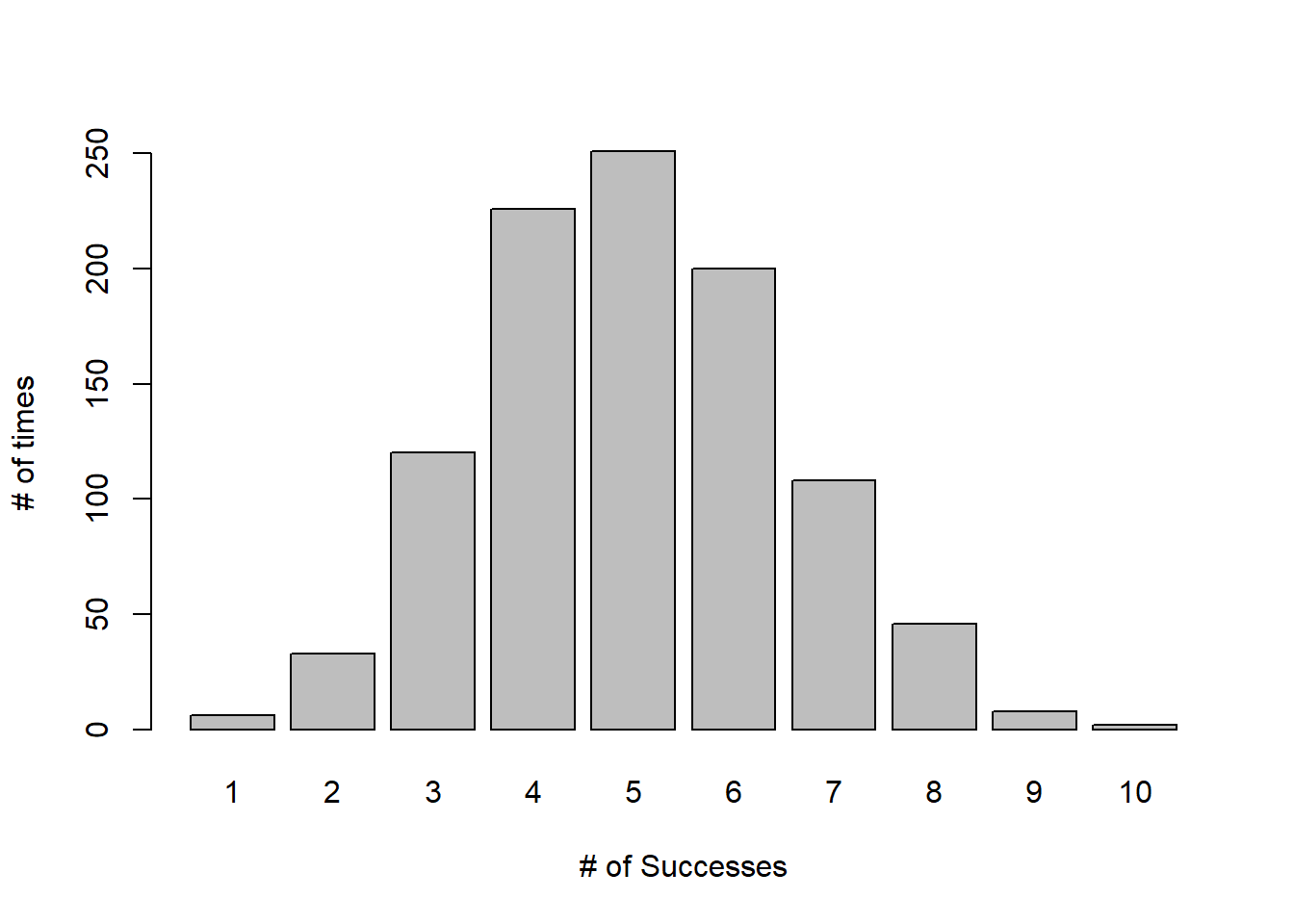
What do you observe?
1.2.5 What is the Probability of a Number of Successes
The results of this experiment will depend greatly on what the true value of \(p\) is. Again, \(p\) is our friend’s probability of guessing correctly.
To start, let’s suppose our friend really can tell the difference between which is added first - 100% of the time - so the probability of success, \(p=1\). How many successes out to 10 attempts would we expect in this case? (Yes, 10.)
Alternatively, let’s suppose she is simply guessing randomly each time. What is the probability she guesses any individual trial correctly? If it’s truly random, then \(p=0.5\), meaning there is a 50% chance she gets it right and a 50% chance she gets it wrong. In that case, what is the probability that she gets exactly 8 correct out of 10 trials? It turns out we can calculate this explicitly.
Let’s define \(Y\) to be a random variable which is the number of successful guesses. (Random variables are like variables in algebra, but the value is uncertain until the event happens.) We can write the probability that she gets exactly 8 correct out of 10 trials if \(p=0.5\) as:
\[P(Y=8|n=10, p=0.5)\]
We’ll read this as the probability of 8 successes given 10 trials and a probability of 50%.
Mathematically we can calculate this as:
\[P(Y=8|n=10, p=0.5) = {10 \choose 8} 0.5^8 0.5^2\]
where \(10\choose 8\) is the “choose” function. The choose function calculates how many different ways can we get 8 successes out of 10 attempts. More on that later as well.
While yes, we could calculate this all by hand, alternatively we could use R to find this more directly as:
## [1] 0.04394531And hence there’s a 4.39% chance she guesses exactly 8 right if \(p=0.5\).
The dbinom() function calculates the probability of a certain number of successes out of a given number of trials for a Binomial distribution with a known \(p\). In this case you can see we are asking about seeing 8 successes out of 10 trials, each with a probability of 0.5.
(Note: this is one of the reasons we will use R this year. It has a large number of built in functions that help us perform statistical analysis.)
1.2.6 Guided Practice
What is the probability that she guesses 8 correct if \(p=0.9\) (i.e. if there’s a 90% chance she can guess correctly)?
Modify and run the above code.
1.2.7 What is the Distribution of Results?
In our experiment, we will observe somewhere between 0 and 10 successes (out of 10 trials), and we can calculate each of these probabilities in a similar manner. We might also plot the distribution of result as:
barplot(dbinom(0:10, 10, 0.5), xlab="# of Successes", ylab="Probability",
        col="lightblue", names.arg=seq(from=0, to=10))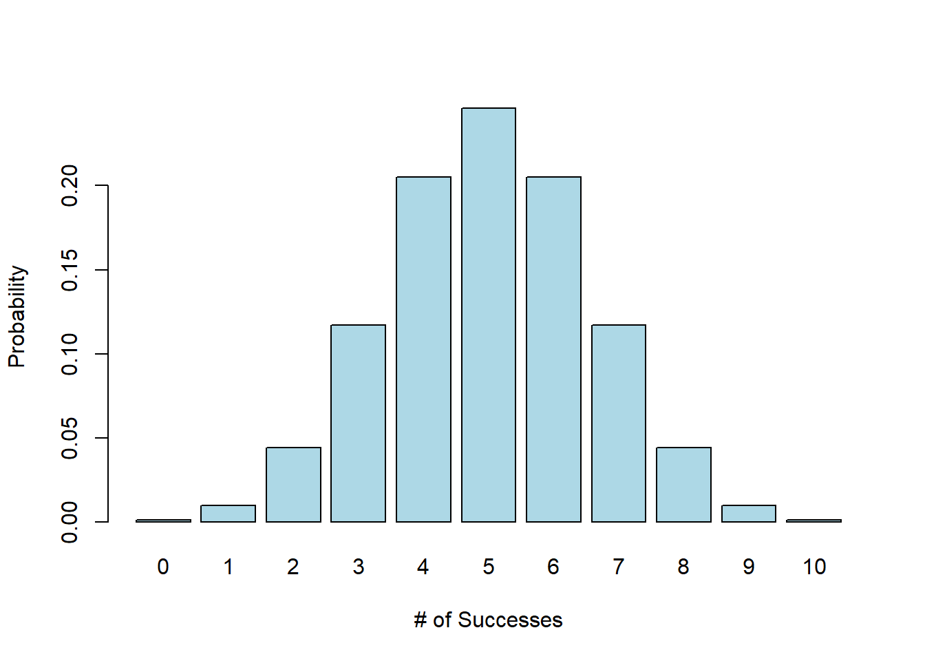
There are a lot of parameters to this plotting function - don’t worry, you’ll learn all those details soon.
Importantly, this is a probability distribution which means it shows us all of the possible outcomes and the probability of each. We’ll see and use a number of different probability distributions this year. Note that the sum of all the probabilities is 1 (or equivalently 100%) because one of these outcomes must occur.
(How is this different from what we did above? Only in one slight way - this is the theoretical/mathematical probability whereas above we saw the simulated results based on our small sample of the class.)
Here, we observe that if \(p=0.5\) (i.e. if she’s simply guessing randomly) our friend is most likely to guess somewhere between 3 and 7 out of 10 correctly. There’s some chance of her randomly getting a result outside of that range, but it’s low.
In fact, \(P(3\le Y \le 7)\) is:
## [1] 0.890625or 89%. The pbinom() function calculates the cumulative probability.
Alternatively, here is the distribution of the number of successes we’d expect if \(p=0.9\) (i.e. she guesses correctly 90% of the time):
barplot(dbinom(0:10, 10, 0.9), xlab="# of Successes", ylab="Probability",
        col="lightblue", names.arg=seq(from=0, to=10))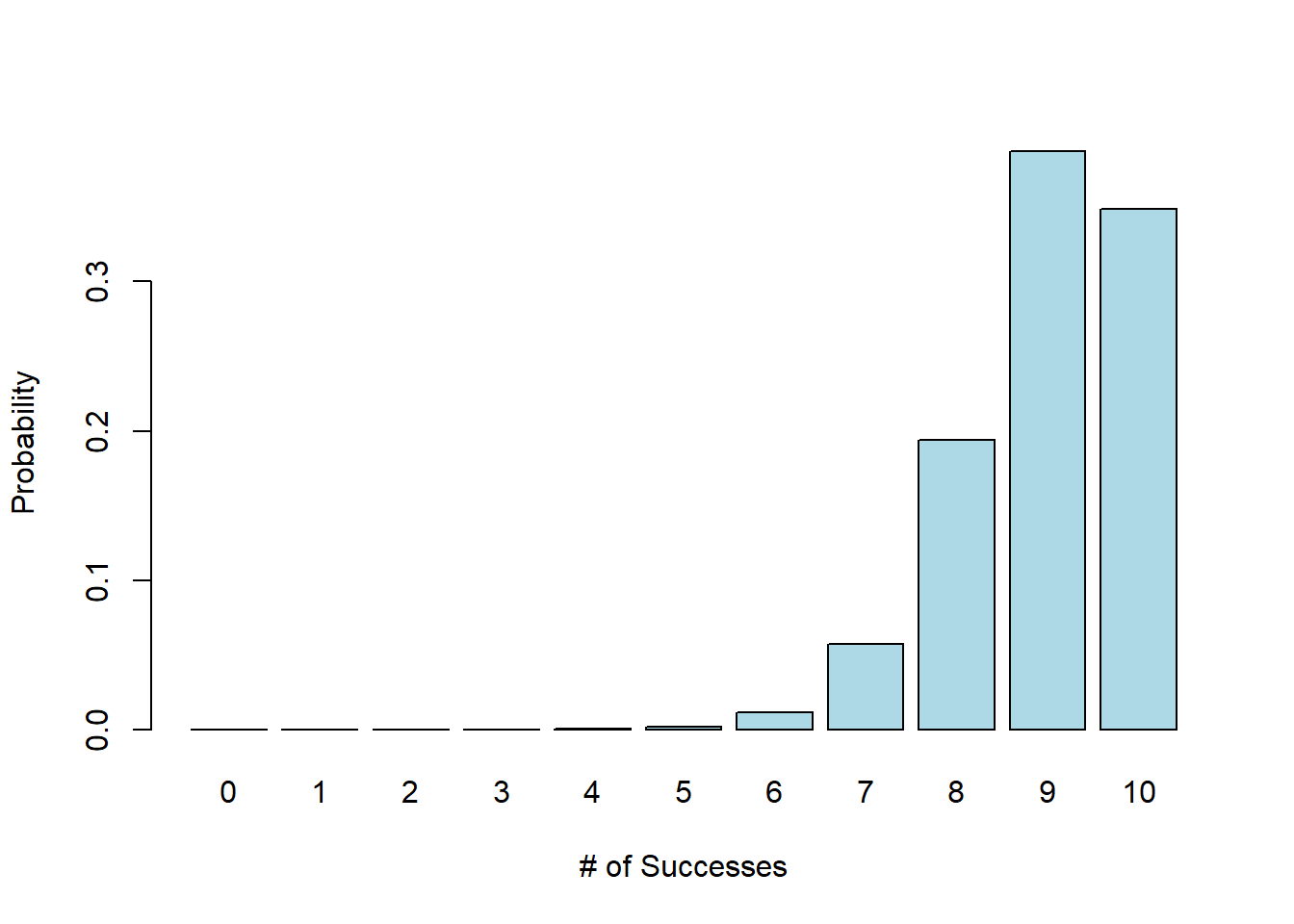
What we see here (which should be what we would expect) is that if \(p=0.9\) (if she’s almost always right), it’s much more likely that our friend would guess 8, 9 or 10 of the trials correctly.
In this case, \(P(8\le Y \le 10)\) is:
## [1] 0.9298092or 93%.
1.3 Running a Hypothesis Test
So, now that we understand something about the expected distribution of results for different values of \(p\), how might we use this to logically evaluate whether our friend can actually distinguish between coffee first or milk first?
Note that when we run our experiment, we only observe \(y\), the number of successes. (I’m using lower case for a specific number whereas upper case is the unknown random variable.) From this we can calculate our sample probability, \(\hat p = \frac{y}{n}\) but we don’t directly observe \(p\), the true probability.
What’s the difference? In theory, there is some true probability of success, but it’s unknowable. Importantly, \(p\) (the true probability) and \(\hat p\) (the sample probability) are not the same. Yes, we’ll use \(\hat p\) to estimate \(p\), and as the number of samples we take gets bigger, \(\hat p\) should get closer to \(p\). The more trials we run, the \(\hat p \rightarrow p\). We’ll learn how to quantify all of this.
OK, back to our question: How might we evaluate whether our friend can actually distinguish between coffee first or milk first?
Maybe we should first decide upon what “can she distinguish” really means?
If the question is: “is she right 100% of the time”, then this becomes somewhat trivial. If \(y \ne 10\), then we know she doesn’t answer correctly 100% of the time. However, what if \(y=10\)? What can we infer in that case? Note: it doesn’t necessarily mean that \(p=1\), because she could get answer all trials correct even if \(p\ne 1\). For example, if \(p=0.85\), \(P(Y=10|n=10, p=0.85)\) is
## [1] 0.1968744Suggesting there’s a 20% chance she get’s them all correct even if \(p=0.85\).
So, if our null hypothesis (our baseline assumption) is that \(p=1\), we see it is easy to reject this hypothesis if she doesn’t answer them all correctly, however, we can’t really confirm this value, even if she does answer them all correctly. This will be a common issue with our statistical tests.
Based on the evidence (she gets them all correct or not), what conclusion is: likely true, possibly true or definitely false?
| result | all correct | not all correct |
|---|---|---|
| \(p=1\)? | ||
| \(p\ne 1\)? |
This is an easier analysis than we typically have, particularly because (as we see) there is one case where we have a definite conclusion.
But what about if our hypothesis is \(p\ne 1\)? We’ll get there in just a second, but first, let’s remind ourselves a bit about logic.
1.3.1 The Logic of our Hypothesis Tests
From geometry you might remember studying logic. For example, if we have a statement: “If \(a\) then \(b\)”, and we observe \(!b\) (not \(b\)), what do we conclude? (Your answer should be \(!a\))
For example, assume we are given the statement: if I drive to school, my car will be in the garage. Then, I observe that my car is not in the garage. The conclusion is therefore that I did NOT drive to school. (Haha, yes, you could have loaned your car to your friend, but then the above statement is no longer true.)
In statistical analysis we’ll take a similar approach, but we need to consider the probability or likelihood of the results.
We’ll use a general framework of
- Statement: If \(a\) then probably \(b\),
- Observation: \(!b\) (not \(b\)),
- Conclusion: Probably not \(a\).
Inherent in this approach are two fundamental concepts. First, we want to know about \(a\), but all we observe is \(b\) and second, there’s some amount of randomness or uncertainty about the results of \(b\) even if \(a\) is true.
1.3.2 What if \(p\ne 1\)?
So back to our coffee and milk example. What about evaluating a different null hypothesis? Maybe our question is whether she’s doing better (or worse!) than simply guessing on each trial. In this case our null hypothesis (our baseline assumption) will be that the true probability \(p=0.5\).
We can then ask what the \(P(Y=y|n=10, p=0.5)\) is for different values of \(y\), the observed number of successes.
Let’s suppose we observe 8 successes. We calculate the \(P(Y=8|n=10, p=0.5)\) as (repeat from above):
## [1] 0.04394531but importantly we don’t typically only look at this when evaluating our hull hypothesis. Instead, we’ll look at \(P(Y\ge8|n=10, p=0.5) = P(Y=8, 9\ or\ 10|n=10, p=0.5)\). What we’re asking here is the probability of seeing results as extreme (or more) than the observed result, if \(H_0\) is true. Why? Because since our null hypothesis is \(p=0.5\), observing 9 or 10 successes would be even less likely, and hence less support for our (null) hypothesis.
We can calculate this probability \(P(Y\ge8|n=10, p=0.5) = P(Y=8)+P(Y=9)+P(Y=10)\) as:
## [1] 0.0546875Suggesting there’s a 5.47% chance of her guessing 8 or more correctly if the true value is \(p=0.5\) (i.e. if she were randomly guessing.)
How should we interpret this value? Again, let’s try to fill in the following table:
| result | less than 8 correct | 8 or more correct |
|---|---|---|
| \(p=0.5\)? | prob\(=0.0547\) | |
| \(p\ne 0.5\)? |
In this case, as we see, unfortunately, none of the conclusions are certain. And whereas I can easily quantify the first row, I’d need more information to quantify the second row.
Also, \(0.05=\frac{1}{20}\) so it means there’s about a 1 in 20 chance she could guess correctly. Is that so unreasonable?
1.4 How Likely is Unlikely?
So, given this uncertainty, what should we conclude about our null hypothesis?
Above we calculated that there is a 5.47% chance that we would see 8 or more successes IF \(p=0.5\). What we need is a threshold that allows us to decide “how likely is unlikely?”
If we calculated that there was only a 1% chance of seeing our observed results if the null hypothesis were true, (i.e. only a 1% chance of her guessing 8 or more correctly if \(p=0.5\)) then we might decide that that is simply too unlikely to occur, and therefore we don’t believe the null hypothesis is true. Alternatively, if we calculated that there was a 30% chance of seeing our observed results (again assuming the null hypothesis were true), then that might be likely enough to cause us to “fail to reject” our null hypothesis.
To reinforce the point, these “chance” values depend on both the observed result (8 successes in this case) and the probability values of the null hypothesis (\(p=0.5\)), so if the overall chance of the observed result is too low, we can infer that the null hypothesis is probably false.
So, what is a good decision threshold to use? The convention in statistics is to use 5% as our threshold. It’s admittedly not perfect. But generally what we’re saying here is that if there is only a 1/20 chance that our observed results could have occurred if the null hypothesis were true, we conclude the null is probably not true. In that case we say we “reject the null hypothesis”.
So in our specific case, we calculated a 5.47% chance of seeing 8 (or more) successes if \(p=0.5\), which isn’t quite unlikely enough to cause us to reject the null hypothesis. So, if she correctly guessed 8 out of 10, we would say we “fail to reject” the null hypothesis that \(p=0.5\), and conclude that we don’t have enough evidence to say she wasn’t simply guessing randomly.
1.4.1 What Happens as \(n\) Increases?
Above, we only tested our friend on 10 cups of coffee. What would have happened if that number were higher, say 20?
If \(p=0.5\) is it harder, easier, or the same to guess 9/10 or 18/20 correct? (both 90% success rates)
## [1] 0.009765625## [1] 0.0001811981What this says is one of our tools (levers?) for improving our tests will be the size of our sample.
1.5 What Actually Happened?
This is actually a true story, sort of.
It was a summer afternoon in Cambridge, England, in the late 1920s. A group of university dons, their wives, and some guests were sitting around an outdoor table for afternoon tea. One of the women was insisting that tea tasted different depending upon whether the tea was poured into the mil or whether the milk was poured into the tea. The scientific minds among the men scoffed at this sheer nonsense. What could be the difference? They could not conceive of any difference in the chemistry of the mixtures that could exist. A thin, short man with thick glasses and a Vandyke beard beginning to turn gray, pounced on the problem.
“Let us test the proposition”, he said excited. He began to outline an experiment in which the lady who insisted there was a difference would be presented with a sequence of cups of tea, in some of which the milk had been poured into the tea and in others of which the tea had been poured in the milk.
Enthusiastically, many of them joined with him in setting up the experiment. Within a few minutes, they were pouring different patterns of infusion in a place where the lady could not see which cup was which. Then, with an air of finality, the man with the Vandyke beard presented her with her first cup. She sipped for a minute and declared that it was one where the milk had been poured into the tea. He noted her response without comment and presented her with the second cup…
From The Lady Tasting Tea: How Statistics Revolutionized Science in the Twentieth Century, David Salsburg, 2001, Holt Publishing, 340pp.
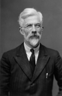
Sir Ronald Fisher
1.6 Key Vocabulary
- true probability of success, \(p\)
- sample proportion, \(\hat p\)
- probability distribution
- Binomial distribution
- random variable
- outcomes
- hypothesis test
- null hypothesis
1.7 Exercises
Exercise 1.1 Above we said that if \(p=1\), we would expect all guesses to be correct. Use the dbinom() function with \(p=1\) to show this is true. Keep the trials at \(n=10\) and evaluate \(y=8\), \(y=9\) and \(y=10\). Why do you see the results that you do?
Exercise 1.2 Above we looked at the probability of 8 or more successes (out of 10) if \(p=0.5\). What is the probability of 8 or more successes if \(p=0.75\)?
Exercise 1.3 Similar to the prior exercise, What is the probability of 16 or more successes if \(p=0.75\) if \(n=20\)? Note that this is the same proportion of successes, however with more trials. Why are the results here different or the same?
Exercise 1.4 We started this chapter by simulating 1000 experiments of \(n=10\) trials with \(p=0.5\).
- Use
rbinom()to simulate 1000 experiments of 12 trials with p=0.2 (now worse than random!)
- Then, create a
barplotthat shows the distribution of the previous simulation. Hint: first store your results from part (a) in a variable and then use thebarplot()command with that variable as a parameter.
1.8 Why Do We Use Statistics?
(Read from The Lady Tasting Tea page 295.)
At the 10,000 ft level, why do we use statistics? Why does this class exist? Is it uncertainty in measurement or uncertainty in data? Is life deterministic? Is it a pool table, where if we knew beforehand, the position of all of the balls and knew the velocity (speed and direction) of the initial impact, could we perfectly predict the outcome (where all balls will stop)?