Chapter 19 Multiple Regression
19.1 Overview
In the previous chapter we looked at simple linear regression, the term “simple” meaning that we only use 1 (one) continuous predictor. In this chapter, we will introduce the idea of multiple linear regression, which allows using multiple continuous and/or categorical predictor variables within the same model.
Linear models require at least one continuous predictor. Why are they called "linear models?" Because, regardless of the number of predictor variables, they retain their linear form, meaning that each new predictor is additive. For example, a model with three continuous predictors (\(X_1, X_2\), and \(X_3\)) might look like:
\[Y = \beta_0 + \beta_1 X_1 + \beta_2 X_2 + \beta_3 X_3 + \epsilon\]
Here \(\beta_0\) is still our intercept, and \(\beta_1, \beta_2\) and \(\beta_3\) are the slope terms for each associated predictor.
In the sections that follow, we will look at how to add both categorical and continuous predictor variables to our model, discuss the approach of model fitting, and how we evaluate and utilize the fitted values.
For using both continuous and categorical variables, we will use the lm() function, however, as we will see, the terms within the function call will change, particularly the formula that describes the linear relationship.
And overall, our approach will mimic what we learned in simple linear regression.
19.2 Using Categorical Predictor Variables
19.2.1 Learning Objectives
Based on this section, you should be able to:
- define what a categorical variable is and discuss why it might be included in a regression model
- understand how our overall null hypothesis changes in multiple regression
- describe the four possible models we might see when using a single categorical variables within multiple regression
- fit alternative models using different formulations within the
lm()function call - interpret the results of a
summary()table for a model with multiple parameters - explain (qualitatively) the role that the
Adjusted R-squaredvalue plays, and discuss why we want a “parsimonious” model. - perform prediction using categorical predictors
19.2.2 Modeling Gas Usage as a Function of Temp and Insulation
We started our simple linear regression discussion (in the previous chapter) with the whiteside data, plotted below:
library(MASS)
plot(whiteside$Temp, whiteside$Gas, xlab="Outside Temp", ylab="Gas Usage", main="Gas usage vs. Outside Temp")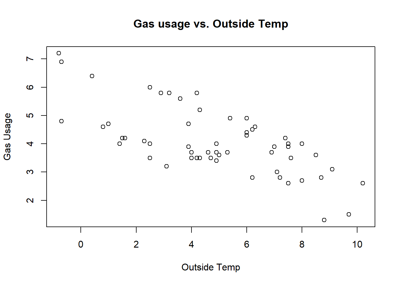
When we first examined the fit of this model, we weren’t in love with the fit, particularly in that none of the observed points were on the fitted line, and the spread of the residuals seemed wider than expected, particularly at lower temperatures. Also, it was unclear if the variance was constant and it didn’t seem that the residuals were necessarily random.
In fact, it turns out there was another variable we didn’t consider:
## [1] "Insul" "Temp" "Gas"The Insul variable is a categorical variable that indicates whether the measurements were taken in the year before or after insulation was installed in the house.
Let’s redo the plot, now showing the points before and after insulation was installed in different colors:
plot(whiteside$Temp, whiteside$Gas, xlab="Outside Temp", ylab="Gas Usage", main="Gas usage vs. Outside Temp", col="dark green")
points(whiteside$Temp[whiteside$Insul=="Before"], whiteside$Gas[whiteside$Insul=="Before"], col="blue")
legend(8,7, c("before", "after"), col=c("blue", "dark green"), pch=1)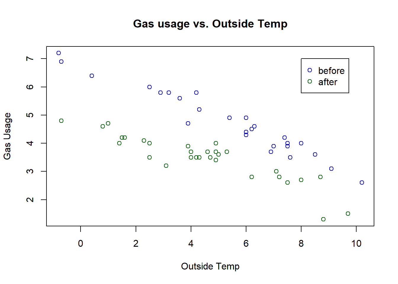
What do you observe? And, based on this pattern, how should we now model this relationship? It is probably clear that a single model (line) isn’t our best option here.
Our first option might be to split this into two different data sets with entirely separate models, but… this would be imprecise, particularly related to our residual error. We’ll discuss the details of that later, and for now, suffice it to say that we can do better.
Conceptually, we know we want to model these two situations differently, but let’s be specific about the math. Our previous model was
\[y= \beta_0 + \beta_1 x + \epsilon\]
In this situation, we probably want different lines to model the before and after situations. But, what specifically would we want to allow to potentially change? Mathematically, we could change \(\beta_0\) or \(\beta_1\) or both.
Maybe it’s easiest to visualize this before describing the equations. Below are four plots with different models shown as lines:

And here are the four possible models (equations), matching what’s shown above:
- Same slope and intercept: \[y = \beta_0 + \beta_1 x + \epsilon\]
- Same slope with different intercept: \[y = (\beta_{00} + I_x\beta_{01}) + \beta_1 x + \epsilon\]
- Different slope and different intercept: \[y = (\beta_{00} + I_x \beta_{01}) + (\beta_{10} + I_x\beta_{11}) x + \epsilon\]
- Different slope and same intercept: \[y = \beta_0 + (\beta_{10} + I_x\beta_{11}) x + \epsilon\]
Note: the indicator function \(I_x\) takes a value of 0 or 1 depending on whether certain data in \(x\) is included or not. So, for example, here it could be \(I_x=0\) for before insulation and \(I_x=1\) for after insulation values. R takes care of the calculations for us, but what you need to recognize is that if \(I_x=1\), the overall slope or intercept of that case will be different.
Given these four possible models:
- Which model seems to “fit” the best?
- Which model makes the most sense, when thinking about the physics of house heating?
These are the questions we need to now evaluate.
However, before we get there, we need to discuss a couple of things. First, how do we get R to model these different situations? Second, how do we evaluate if any of these are a “good” fit?
To address the first question, to fit these different models in R, we’ll simply change the formula of our model within the lm() call.
- One line - same slope and intercept (this is the same model we previously used and here we are ignoring whether insulation exists or not):
##
## Call:
## lm(formula = Gas ~ Temp, data = whiteside)
##
## Residuals:
##     Min      1Q  Median      3Q     Max
## -1.6324 -0.7119 -0.2047  0.8187  1.5327
##
## Coefficients:
##             Estimate Std. Error t value Pr(>|t|)
## (Intercept)   5.4862     0.2357  23.275  < 2e-16 ***
## Temp         -0.2902     0.0422  -6.876 6.55e-09 ***
## ---
## Signif. codes:  0 '***' 0.001 '**' 0.01 '*' 0.05 '.' 0.1 ' ' 1
##
## Residual standard error: 0.8606 on 54 degrees of freedom
## Multiple R-squared:  0.4668, Adjusted R-squared:  0.457
## F-statistic: 47.28 on 1 and 54 DF, p-value: 6.545e-09- Two lines - same slope with different intercept (we’ve added
Insulas a predictor):
##
## Call:
## lm(formula = Gas ~ Temp + Insul, data = whiteside)
##
## Residuals:
##      Min       1Q   Median       3Q      Max
## -0.74236 -0.22291  0.04338  0.24377  0.74314
##
## Coefficients:
##             Estimate Std. Error t value Pr(>|t|)
## (Intercept)  6.55133    0.11809   55.48   <2e-16 ***
## Temp        -0.33670    0.01776  -18.95   <2e-16 ***
## InsulAfter  -1.56520    0.09705  -16.13   <2e-16 ***
## ---
## Signif. codes:  0 '***' 0.001 '**' 0.01 '*' 0.05 '.' 0.1 ' ' 1
##
## Residual standard error: 0.3574 on 53 degrees of freedom
## Multiple R-squared:  0.9097, Adjusted R-squared:  0.9063
## F-statistic: 267.1 on 2 and 53 DF,  p-value: < 2.2e-16
What’s interesting (new) about this output is the InsulAfter term. This represents how much the intercept changes for all values where Insulation ==“After”.
So, our two different lines are: before insulation is \(y= 6.55 - 0.337*x\) and after insulation is \(y= (6.55-1.56) - 0.337*x = 4.99 - 0.337*x\). Notice that the two equations have the same slope but different intercepts.
- Two lines - different slope and different intercept (we’re now allowing for an interaction between
TempandInsul):
##
## Call:
## lm(formula = Gas ~ Temp * Insul, data = whiteside)
##
## Residuals:
##      Min       1Q   Median       3Q      Max
## -0.97802 -0.18011  0.03757  0.20930  0.63803
##
## Coefficients:
##                 Estimate Std. Error t value Pr(>|t|)
## (Intercept)      6.85383    0.13596  50.409  < 2e-16 ***
## Temp            -0.39324    0.02249 -17.487  < 2e-16 ***
## InsulAfter      -2.12998    0.18009 -11.827 2.32e-16 ***
## Temp:InsulAfter  0.11530    0.03211   3.591 0.000731 ***
## ---
## Signif. codes:  0 '***' 0.001 '**' 0.01 '*' 0.05 '.' 0.1 ' ' 1
##
## Residual standard error: 0.323 on 52 degrees of freedom
## Multiple R-squared:  0.9277, Adjusted R-squared:  0.9235
## F-statistic: 222.3 on 3 and 52 DF,  p-value: < 2.2e-16
What’s new about this output is the Temp:InsulAfter term. This represents how much the slope changes for all values where Insulation ==“After”.
So, our two different lines are: before insulation is \(y= 6.854 - 0.393*x\) and after insulation is \(y= (6.854-2.130) + (-0.393 +0.115)*x = 4.724 - 0.278*x\). Notice that these two equations have different slopes and different intercepts.
- Two lines - different slope and same intercept (similar to above, but we’re restricting the interaction to just be a different slope):
##
## Call:
## lm(formula = Gas ~ Temp:Insul, data = whiteside)
##
## Residuals:
##      Min       1Q   Median       3Q      Max
## -1.14216 -0.46461 -0.03467  0.42504  1.38776
##
## Coefficients:
##                  Estimate Std. Error t value Pr(>|t|)
## (Intercept)       5.63978    0.16965  33.244  < 2e-16 ***
## Temp:InsulBefore -0.21557    0.03184  -6.771 1.06e-08 ***
## Temp:InsulAfter  -0.43198    0.03590 -12.034  < 2e-16 ***
## ---
## Signif. codes:  0 '***' 0.001 '**' 0.01 '*' 0.05 '.' 0.1 ' ' 1
##
## Residual standard error: 0.6146 on 53 degrees of freedom
## Multiple R-squared:  0.7331, Adjusted R-squared:  0.7231
## F-statistic:  72.8 on 2 and 53 DF,  p-value: 6.268e-16
What’s new about this output is the Temp:InsulBefore term and the lack of a slope term. Here the Temp:InsulBefore value is the slope when Insulation ==“Before” and the Temp:InsulAfter value is the slope when Insulation ==“After”.
So, our two different lines are: before insulation is \(y= 5.640 - 0.216*x\) and after insulation is \(y= 5.640 -0.432*x\).
19.2.3 Possible models with Categorical Variables
Here is a summary of the different models we might select from.
| Description | Model | R command |
|---|---|---|
| same slope and intercept | \(y = \beta_0+ \beta_1 x +\epsilon\) | lm(Gas~Temp, data=whiteside) |
| same slope, different intercept | \(y = (\beta_{00} + I_x\beta_{01}) + \beta_1 x + \epsilon\) | lm(Gas~Temp+Insul, data=whiteside) |
| different slope, different intercept | \(y = (\beta_{00} + I_x \beta_{01}) + (\beta_{10} + I_x\beta_{11}) x + \epsilon\) | lm(Gas~Temp*Insul, data=whiteside) |
| different slope, same intercept | \(y = \beta_0 + (\beta_{10} + I_x\beta_{11}) x + \epsilon\) | lm(Gas~Temp:Insul, data=whiteside) |
19.2.4 How Should we Interpret the Models?
When thinking about whether a model is a good fit, it’s important to consider the relationship between model formulas and what the variables within the model physically represent about their interactions.
First, let’s consider the model with different intercepts but same the slope (figure and model b). What this model suggests is that the relationship between the temperature and gas usage is constant (same slope), and the insulation just adjusts the starting point.
Next, consider the model with different intercepts AND different slopes (figure and model c). What this model suggests is that the relationship between the temperature and gas usage is different (same slope) when insulation is present or not. In this case, there is interaction between the variables and our model doesn’t assume they are acting independently.
To decide between such models we’d probably need a building materials expert to help us understand which of these models makes the most sense from a heat flow perspective. However, we can still use statistics to look at which model “fits” the best.
19.2.5 Does Each Model Fit Well?
In fact, before we compare model fits, we would follow a similar approach as we did in the previous chapter to ensure a linear model is appropriate in each case. Even though we’ve added a new predictor, the same assumptions still hold. Specifically, for each proposed model, we should look at:
- The plot of the data and fitted lines. Is the relationship between \(x\) and \(y\) for each group linear?
- The distribution of the residuals. We still need to ensure no trend exists in the residuals and that they are roughly distributed \(N(0, \epsilon)\)
- Whether all of the parameters, including any offsets to the slope or intercept, are significantly different than 0.
Per the last bullet, for models with multiple slope or intercept parameters, we need confirm that such parameters are “significant” (i.e. significantly different from 0). We do this as before, however modified slightly since there are said additional parameters to consider. For example, here is the summary output for model c:
##
## Call:
## lm(formula = Gas ~ Temp * Insul, data = whiteside)
##
## Residuals:
##      Min       1Q   Median       3Q      Max
## -0.97802 -0.18011  0.03757  0.20930  0.63803
##
## Coefficients:
##                 Estimate Std. Error t value Pr(>|t|)
## (Intercept)      6.85383    0.13596  50.409  < 2e-16 ***
## Temp            -0.39324    0.02249 -17.487  < 2e-16 ***
## InsulAfter      -2.12998    0.18009 -11.827 2.32e-16 ***
## Temp:InsulAfter  0.11530    0.03211   3.591 0.000731 ***
## ---
## Signif. codes:  0 '***' 0.001 '**' 0.01 '*' 0.05 '.' 0.1 ' ' 1
##
## Residual standard error: 0.323 on 52 degrees of freedom
## Multiple R-squared:  0.9277, Adjusted R-squared:  0.9235
## F-statistic: 222.3 on 3 and 52 DF,  p-value: < 2.2e-16
Looking at the coefficients table, we see four rows to consider. In this case we note that all of the coefficient estimates (for this model) are significantly different than 0 (i.e. all p-values much less than 0.05).
This is an important step as we don’t want to have models with coefficients that aren’t significant.
19.2.6 What is the Overall Null Hypothesis?
When we consider multiple regression, our overall null hypothesis changes slightly. For any given model, we have:
- \(H_0\): that none of the coefficients are significantly different than zero.
- \(H_A\): that at least one of the coefficients is significantly different than zero.
As we look at the previous model fit and summary output, we see the last line says: p-value: < 2.2e-16. This p-value refers to the overall model, and so in this case we would conclude that at least one of the fitted coefficients is different than 0. Generally I find this less useful than looking at the individual coefficient values.
19.2.7 How do we Decide which Model is Best?
Now, assuming we’ve gone through and decided that a linear model is appropriate for each of the possible models (or at least some set of possible models do), how do we choose between them?
The next step is to decide which model is “best”? Statistical analysis can only answer part of this. As discussed above, any model needs to be well reasoned out, including the physics of heat flow or whatever is appropriate for the context of the problem.
Assuming so, (and admittedly sometimes we don’t know) one approach to compare models is to look at which model has the most explanatory power, i.e. which one explains more of the variation in \(y\). We previously use \(R^2\) to evaluate this. Here, we will use the adjusted \(R^2\), which provides a similar result.
Here is a comparison of our models with the number of parameters and adjusted \(R^2\) values shown:
| Model | # of parameters | Adjusted \(R^2\) |
|---|---|---|
| same slope and intercept | 2 | 0.457 |
| same slope, different intercept | 3 | 0.9063 |
| different slope, same intercept | 3 | 0.7231 |
| different slope, different intercept | 4 | 0.9235 |
Adjusted \(R^2\) takes the general \(R^2\) value we previously discussed, and then lowers it based on the number of parameters in the model. We basically penalize our results to ensure they’re valid and that we aren’t adding many unnecessary predictors in an attempt to make \(R^2\) as large as possible.
Overall, our goal in multiple regression is to create a “parsimonious” model, which is one that has as few as predictors as possible and still has good explanatory power.
So, based on all of this, I’d argue that the model with the different slope and different intercept is the best, as it has the highest adjusted \(R^2\), even though it has one more parameter.
19.2.8 Guided Practice
Imagine you have a data set that tracks students test scores, the amount they study (in hours) and their grade level for high schoolers, (freshman, sophomores, juniors and seniors). Assume scores, study and grade are the three variable names.
- What are the best predictor and response variable(s)?
- If we want to model
scoresas a function of hours studied and grade level, which is our continuous predictor and which is the categorical predictor? - Assuming you want a model with the same overall slope but different intercepts per grade, how many total parameters would your model have? How would you write this
lm()call? - Assuming you want a model with the different slope and intercepts per grade, how many total parameters would your model have? How would you write this
lm()call?
19.2.9 What about Prediction?
Let’s suppose we wanted to predict the gas usage at a temperature of 5 after insulation has been installed. How would we that?
First, we need to know which model? Let’s use the model with separate slopes and intercepts.
##
## Call:
## lm(formula = Gas ~ Temp * Insul, data = whiteside)
##
## Residuals:
##      Min       1Q   Median       3Q      Max
## -0.97802 -0.18011  0.03757  0.20930  0.63803
##
## Coefficients:
##                 Estimate Std. Error t value Pr(>|t|)
## (Intercept)      6.85383    0.13596  50.409  < 2e-16 ***
## Temp            -0.39324    0.02249 -17.487  < 2e-16 ***
## InsulAfter      -2.12998    0.18009 -11.827 2.32e-16 ***
## Temp:InsulAfter  0.11530    0.03211   3.591 0.000731 ***
## ---
## Signif. codes:  0 '***' 0.001 '**' 0.01 '*' 0.05 '.' 0.1 ' ' 1
##
## Residual standard error: 0.323 on 52 degrees of freedom
## Multiple R-squared:  0.9277, Adjusted R-squared:  0.9235
## F-statistic: 222.3 on 3 and 52 DF,  p-value: < 2.2e-16
Given the above output, how would we use the following equation for prediction?
\[y = (\beta_{00} + I_x \beta_{01}) + (\beta_{10} + I_x\beta_{11}) * x\]
We would have: (i) to pull the appropriate coefficient values out of the summary table and (ii) figure out a value for \(x\). Given \(x=5\) (as posed in the problem), we have:
## [1] 3.334Suggesting our best (point) estimate of the gas usage for a house after insulation has been installed at a temperature of 5 degrees is 3334 cu ft per week.
Of course, we could do this more easily with the predict function, and moreover, more than just a point estimate we want an interval. The only challenge here is to setup the newx variable correctly, which now needs values of both Temp and Insul:
newx <- data.frame(Temp=c(5), Insul=c("After"))
predict(whiteside.lm3, newdata=newx, interval="prediction")
## fit lwr upr
## 1 3.334175 2.674843 3.993507which suggests we’d see a heating gas usage ranging between 2675 and 3994 cubic feet per week.
And let’s plot this so we see a visual of what’s happening:
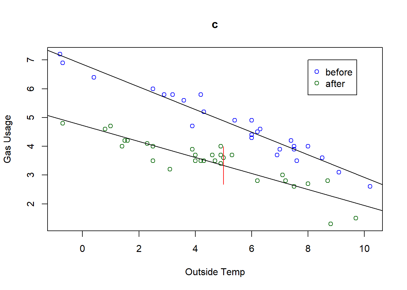
The red vertical line shows the range of expected values for a prediction at Temp=5 “After” insulation.
19.2.10 Summary and Review
Based on this section, you should be able to:
- define what a categorical variable is and discuss why it might be included in a regression model
- understand how our overall null hypothesis changes in multiple regression
- describe the four possible models we might see when using a single categorical variables within multiple regression
- fit alternative models using different formulations within the
lm()function call - interpret the results of a
summary()table for a model with multiple parameters - perform prediction using categorical and continuous predictors
- explain (qualitatively) the role that the
Adjusted R-squaredvalue plays, and discuss why we want a “parsimonious” model.
19.3 Multiple Continuous Predictor Variables
In this section, we will discuss how to create and analyze regression models with multiple continuous variables.
19.3.1 Learning Objectives
Based on this section, you should be able to:
- explain how we can use multiple continuous variables within linear regression models
- fit alternative models using different formulations within the
lm()function call - interpret the results of a
summary()table for a model with multiple continuous predictors (and associated coefficients) - explain qualitatively the role that an adjusted \(R^2\) value plays, and understand issues around model selection.
- evaluate the assumptions of multiple regression, and in particular make residual plots
- make predictions for models with multiple predictors
19.3.2 Multiple Regression with Continuous Predictors
The following is a data set about 50 different startups download from Kaggle (https://www.kaggle.com/). The overall goals here is to see if we can create a model of profit for these startups as a function of other business expenses.
## [1] "R.D.Spend"       "Administration"  "Marketing.Spend" "State"
## [5] "Profit"
I don’t like the built in names so I’m going to change them…
And I should probably quickly define these:
RnD= Research and Development costs are typically engineering costs that occur during product development. It may include payroll costs of engineering staff along test equipment, computers, etc.Admin= Administration costs are typically overhead functions, like payroll, rent, etc.- Marketing costs are related to product advertising.
- State is the US state that the company operates in, either NY, CA or FL.
- Profit is typically ‘net’, meaning that its income minus expenses.
Note that with accounting designations there’s some flexibility as to how expenses are classified. Different companies may account for things slightly differently so there may be some additional variability here.
As far as the States, let’s confirm which states are included in this data set:
## [1] "New York" "California" "Florida"Here are the first few rows of the data:
##        RnD     Admin Marketing      State   Profit
## 1 165349.2 136897.80  471784.1   New York 192261.8
## 2 162597.7 151377.59  443898.5 California 191792.1
## 3 153441.5 101145.55  407934.5    Florida 191050.4
## 4 144372.4 118671.85  383199.6   New York 182902.0
## 5 142107.3  91391.77  366168.4    Florida 166187.9
## 6 131876.9  99814.71  362861.4   New York 156991.1
19.3.3 Exploratory Data Analysis
Let’s plot this data. I’m going to plot all of the data at the same time here by simply calling plot():
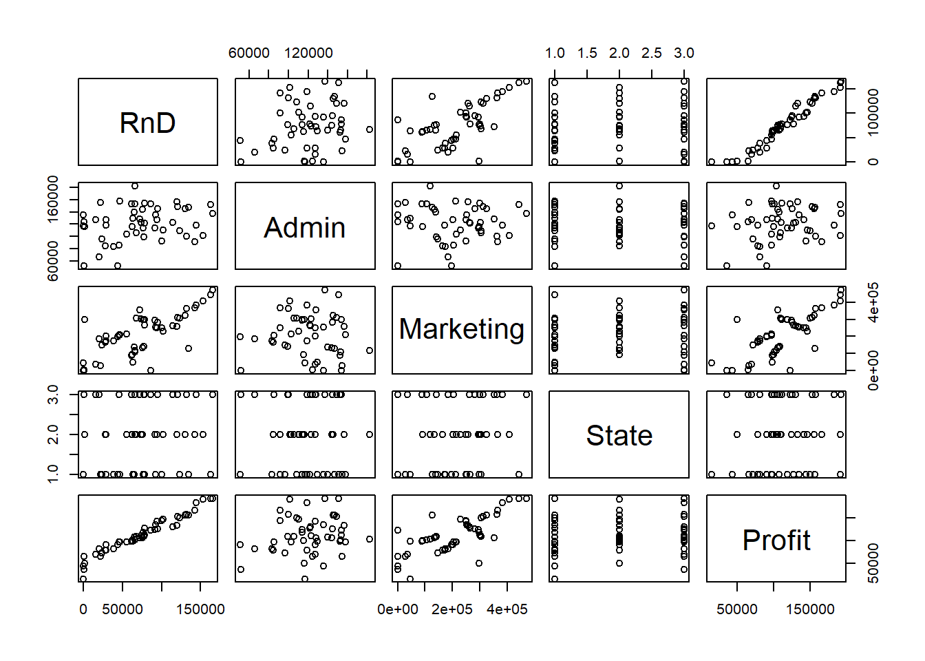
How to read this graph? For the plots in the first row, they all have RnD on the y-axis. For the plots in the third column, they all have Marketing on the x-axis. And so forth.
So what do we observe? Remembering that we are attempting to see if any of these variables might be a good predictor of Profit.
RnDseems to be strongly, positively correlated withProfit.Marketingseems to be weakly, positively correlated withProfit.Adminmay not be correlated withProfitat all.
Now, let’s expand the two most obvious ones:
par(mfrow=c(1,2))
plot(startup$RnD, startup$Profit, xlab="Research & Development", ylab="Profit")
plot(startup$Marketing, startup$Profit, xlab="Marketing", ylab="Profit")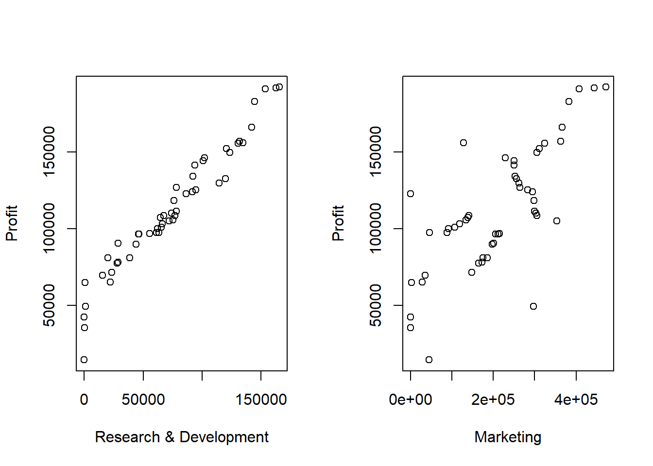
As we did previously, how would you interpret these relationships?
19.3.4 Multicollinearity
One possible issue we need to watch out for when doing multiple regression is whether multicollinearity exists between predictor variables. Basically we don’t want different predictor variables to be highly correlated with one another. This will weaken the statistical significance we assign to any given predictor variable. For now, the important part is simply thta you know of this potential issue.
19.3.5 Modeling Profit
What we’d now like to do is create a model of profit as a function of these other variables. Given the plots, we’ve said the most likely choices of predictor variables are RnD and Marketing. But, how do we create a model that includes both of these at the same time?
Our “general” multiple linear regression model is:
\[y = \beta_0 + \beta_1 x_1 + \beta_2 x_2 + \beta_3 x_3 + \cdots + \epsilon\]
where \(x_1, x_2, x_3, \cdots\) are the different predictor variables and \(\beta_0, \beta_1, \beta_2, \beta_3, \cdots\) are the associated coefficients.
What’s new here is we’re adding additional predictors and their coefficients.
When we say it’s “linear”, we mean it’s linear in the predictors, each new variable has it’s own slope and is additive to the overall model.
So, if we are going to create a model of Profit \(y\) as a function of both RnD \(x_1\) and Marketing \(x_2\) we’ll only use some of the terms above.
And note that \(\epsilon\) is still there. We still make the same assumptions about the residuals: random, constant variance, and normally distributed.
19.3.6 Visualizing Multiple Linear Regression
How might we visualize this situation? With a single predictor we have a fitted line. What do we have with two predictors? We have a fitted plane!
Let’s imagine this in 3D: Put the response variable on the \(z\) axis and our two predictors on the \(x\) and \(y\) axis. However, since our model is that \(y\) is a function of \(x_1\) and \(x_2\), we’ll replace \(z\) with \(y\) and \(y\) with \(x_2\).
The equation of a plane in our statistical notation is \[y = \beta_0 + \beta_1 x_1 + \beta_2 x_2\]
See the following diagram. Here the green points represent observed data and the blue points are the fitted values, which by design fall right on the plane. As we saw with simple regression, some observed values are above the plane and some are below.
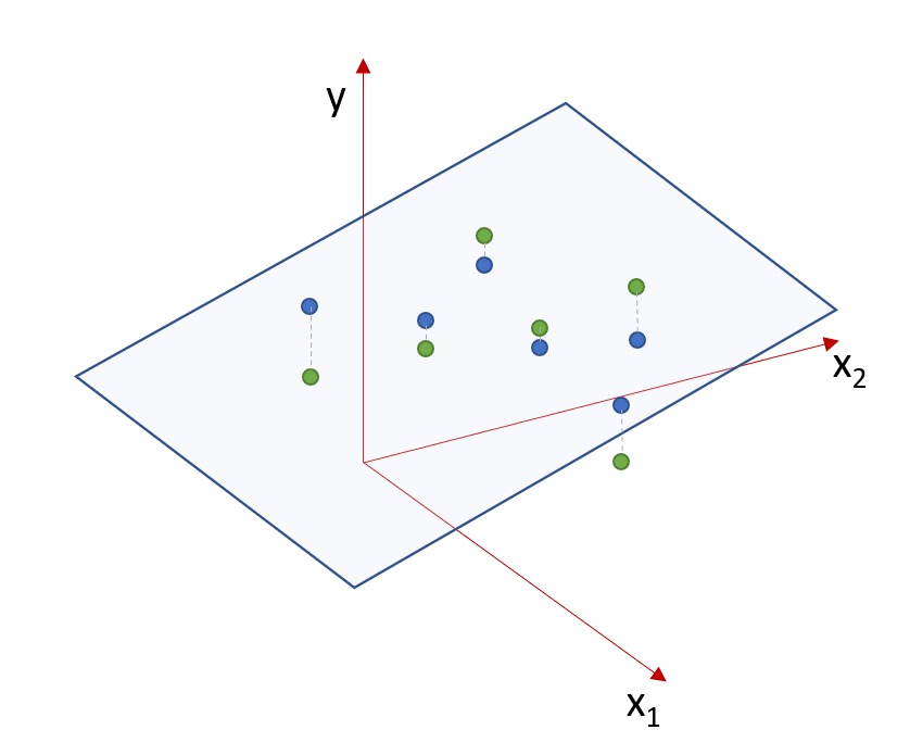
Figure 19.1: The fitted plane for multiple regression analysis.
Again here, the residuals are going to be the distance (in the vertical \(y\) direction) each observed point lies away from the fitted plane. Here residuals are shown as dashed gray lines. As with simple linear regression, the best fitted plane (and hence the values of the coefficients) is one that minimizes the sum of the square of the residuals.
As you can probably imagine, visualizing more than 3 dimensions (2 predictor variables) becomes pretty complicated, however, modeling additional predictors in R is not too difficult.
19.3.7 Modeling Profit in R
Similar to what we did with categorical predictors, we can simply change our lm() call to include additional predictors, using the + sign within the model formula. Here is a possible model of profit we might consider, which also includes Admin as a predictor and the associated summary() output.
##
## Call:
## lm(formula = Profit ~ RnD + Marketing + Admin, data = startup)
##
## Residuals:
##    Min     1Q Median     3Q    Max
## -33534  -4795     63   6606  17275
##
## Coefficients:
##               Estimate Std. Error t value Pr(>|t|)
## (Intercept)  5.012e+04  6.572e+03   7.626 1.06e-09 ***
## RnD          8.057e-01  4.515e-02  17.846  < 2e-16 ***
## Marketing    2.723e-02  1.645e-02   1.655    0.105
## Admin       -2.682e-02  5.103e-02  -0.526    0.602
## ---
## Signif. codes:  0 '***' 0.001 '**' 0.01 '*' 0.05 '.' 0.1 ' ' 1
##
## Residual standard error: 9232 on 46 degrees of freedom
## Multiple R-squared:  0.9507, Adjusted R-squared:  0.9475
## F-statistic:   296 on 3 and 46 DF,  p-value: < 2.2e-16
Note in this case we have four coefficients: \(\beta_0\) (the intercept), \(\beta_1\) (the slope for RnD), \(\beta_2\) (the slope for Marketing), and \(\beta_3\) (the slope for Admin).
What do you observe? Which predictors are significant?
Key things to look for when analyzing a summary() output for multiple regression include:
- what is the overall p-value of our test (and what is our \(H_0\))?
- which of the variables are significant?
- what is the overall
Adjusted R-squared?
To the first point, the last line of the summary output shows p-value: < 2.2e-16. When we are running at multiple regression, our null hypothesis is slightly different than previous. In particular, our null hypothesis here is that at least one of the coefficients is different than zero. We then need to refer back to the coefficient table to figure out which ones are.
19.3.8 Interpreting the Coefficients
What do the coefficients \(\beta_1, \beta_2\) and \(\beta_3\) represent?
A dollar increase in RnD spending will result in a $0.806 increase in profit, all other variables held constant. We might also say, for marketing budget and admin costs held constant.
A dollar increase in Marketing spending will result in a $0.0272 increase in profit, all other variables held constant.
A dollar increase in Admin spending will result in a $0.0268 decrease (because its negative) in profit, all other variables held constant.
The (Intercept) (\(\beta_0\)) still retains a similar meaning. Here its the predicted profit if RnD, Marketing and Admin are all zero. This is another example of where it helps locates the surface, but is a bit nonsensical in itself. How could you have profit if all of those were zero?
19.3.9 Inspecting the Residuals
Ok, so we’ve fit a model, but before we decide we’re too happy with it, we need to make sure our assumptions are satisfied. Primarily we’ll look at the residual plot.
Here is a residual plot, and notice now I’m using the fitted values as the \(x\) variable.
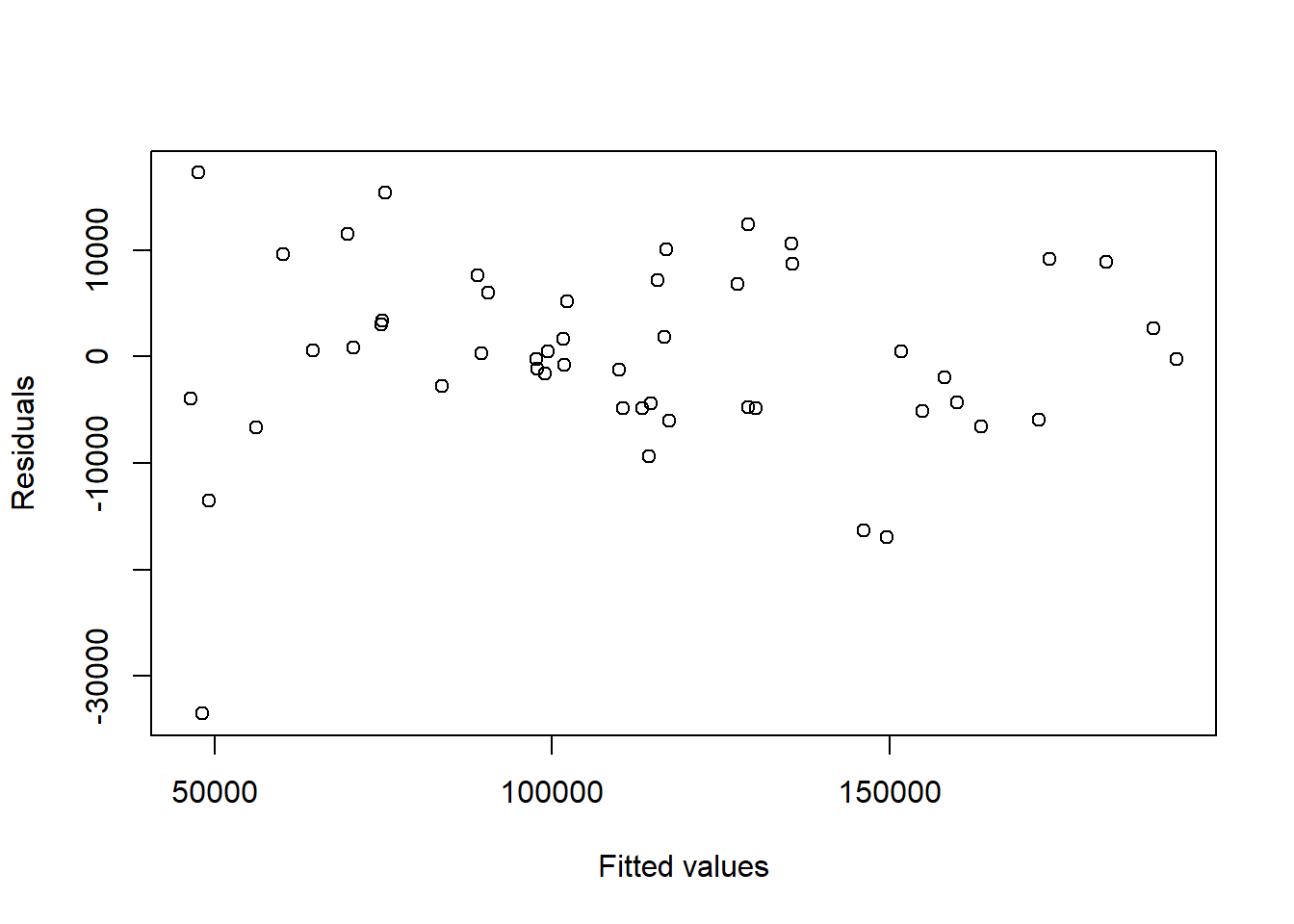
What do you observe? It looks OK except for that one value with a residual below -30000. How do we figure out which point that is? I can use something like:
## 50
## 50
which tells me it’s the 50th point in our data set:
##    RnD    Admin Marketing      State  Profit
## 50   0 116983.8  45173.06 California 14681.4
And maybe what’s odd here is that this company spend $0 on Research and Development?
We could use a similar approach to inspect the companies that have residuals which are greater than 15000 in absolute value:
## 15 16 50
## 15 16 50## 37 46
## 37 46Based on this, we find points 15, 16, 37 46 and 50 to be slightly suspect. We might want to inspect these points further to understand why.
##          RnD    Admin Marketing      State    Profit
## 15 119943.24 156547.4 256512.92    Florida 132602.65
## 16 114523.61 122616.8 261776.23   New York 129917.04
## 37  28663.76 127056.2 201126.82    Florida  90708.19
## 46   1000.23 124153.0   1903.93   New York  64926.08
## 50      0.00 116983.8  45173.06 California  14681.40
19.3.10 What if we added more predictors?
Just to demonstrate, we could evaluate if there is a difference in profitability by State? Note that State is a categorical predictor variable, but we treat it the same.
Of course we should first plot Profit as a function of State using:
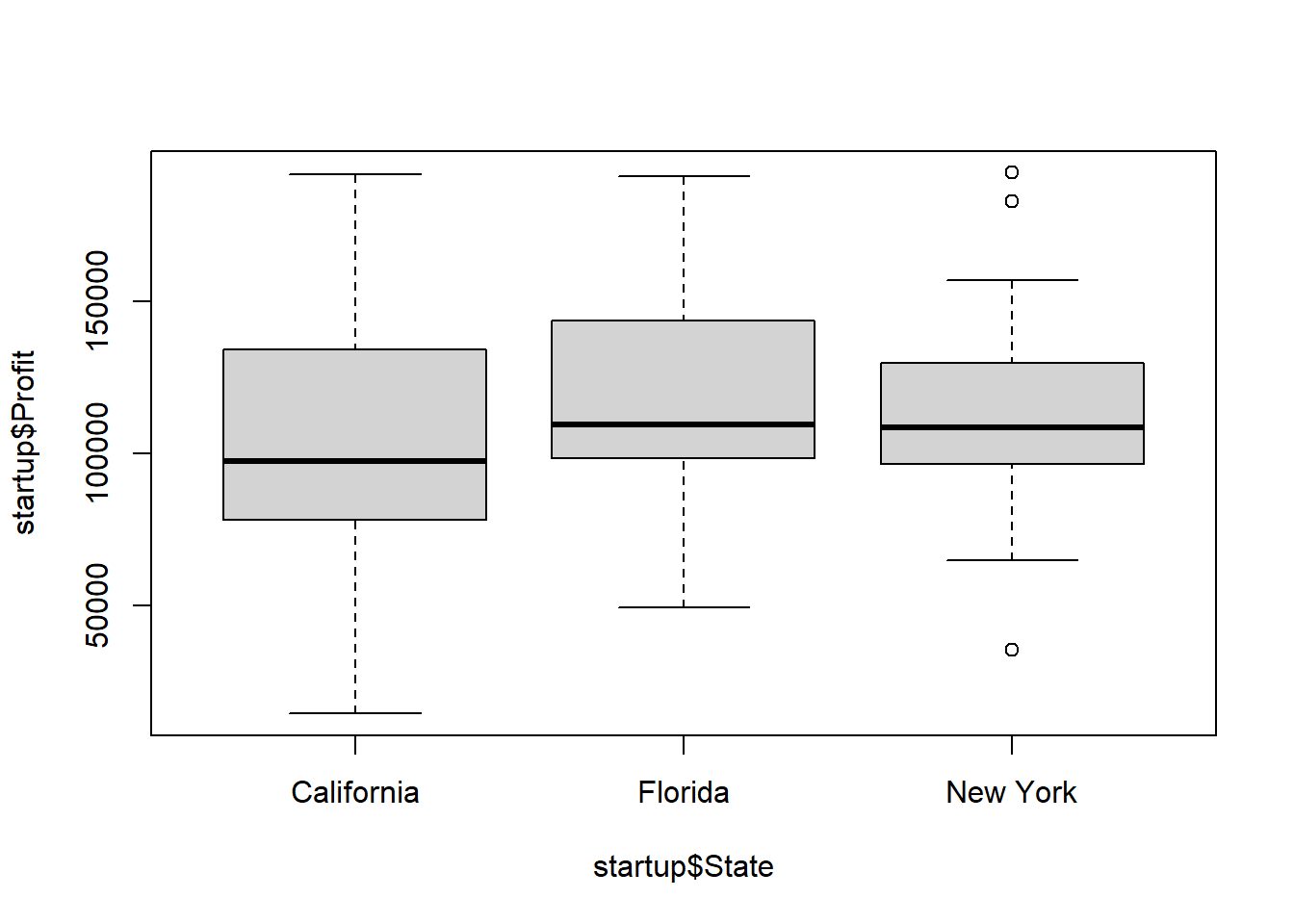
It’s not obvious that this is a useful predictor, but let’s add it to our model and see:
##
## Call:
## lm(formula = Profit ~ RnD + Marketing + Admin + State, data = startup)
##
## Residuals:
##    Min     1Q Median     3Q    Max
## -33504  -4736     90   6672  17338
##
## Coefficients:
##                 Estimate Std. Error t value Pr(>|t|)
## (Intercept)    5.013e+04  6.885e+03   7.281 4.44e-09 ***
## RnD            8.060e-01  4.641e-02  17.369  < 2e-16 ***
## Marketing      2.698e-02  1.714e-02   1.574    0.123
## Admin         -2.700e-02  5.223e-02  -0.517    0.608
## StateFlorida   1.988e+02  3.371e+03   0.059    0.953
## StateNew York -4.189e+01  3.256e+03  -0.013    0.990
## ---
## Signif. codes:  0 '***' 0.001 '**' 0.01 '*' 0.05 '.' 0.1 ' ' 1
##
## Residual standard error: 9439 on 44 degrees of freedom
## Multiple R-squared:  0.9508, Adjusted R-squared:  0.9452
## F-statistic: 169.9 on 5 and 44 DF,  p-value: < 2.2e-16
R has now added two new coefficients: StateFlorida and StateNew York. What do those each represent? You might refer back to the previous section if this isn’t clear.
19.3.11 Comparing Models and Model Selection
So how do we choose the “best” model?
Here’s a summary table of a variety of different models, all including RnD as well as other possible predictors. The adjusted \(R^2\) values for the model are included along with the number of coefficients (don’t forget about the intercept!):
| Profit~ | # of Coefficients | Adjusted \(R^2\) |
|---|---|---|
| RnD + Marketing + Admin | 4 | 0.9475 |
| RnD + Marketing + Admin + State | 5 | 0.9452 |
| RnD + Marketing | 3 | 0.9483 |
| RnD | 2 | 0.9454 |
Based on this table, we find the model that has just RnD and Marketing is the best model as it has the highest adjusted R-squared value.
Note: Model selection can get very complicated as the number of predictors goes up!
19.3.12 What about Prediction
Now that we have chosen our best model, how much profit would we predict for a company with an R&D budget of $100k, a Marketing budget of $25k, Admin expenses of $120k, located in California?
Here is the model declaration:
Note that since our best model does NOT include Admin or State, we won’t actually use that information in our prediction.
Our steps for using R to predict include (same as before):
- Make sure your model has the right form,
- Setup your
newxdata.frame to include values for all relevant predictors, and - Call the
predictfunction using the model,newxand the type of prediction you want.
Here is the process in R code:
newx <- data.frame(RnD=c(100000), Marketing=c(25000))
predict(startup.lm3, newx, interval="prediction")
## fit lwr upr
## 1 127382 107298.6 147465.3So our best estimate is a profit of $127,382 with a 95% confidence interval of {107,298, 147,465}.
19.3.13 Review of our Steps
Generally, here are the steps for multiple regression:
- Explore the data with plots and other statistical analysis
- Fit some models and look at significance of predictors and adjusted \(R^2\)
- Choose best fitting model
- Evaluate the residuals and other assumptions
- Use the model to make predictions
19.3.14 Assumptions about Multiple Linear Regression
- The relationship between the response and predictor data is linear
- There is no multicollinearity in the data
- The values of the residuals are independent of one another
- The variance of the residuals is constant
- The residuals are normally distributed
19.3.15 Summary and Review
Based on this lecture, you should be able to:
- explain how we can use both categorical and continuous variables in multiple regression models
- fit alternative models using different formulations within the
lm()function call - interpret the results of a
summary()table for a model with multiple continuous predictors (and associated coefficients) - explain qualitatively the role that an adjusted \(R^2\) value plays, and understand issues around model selection.
- evaluate the assumptions of multiple regression, and in particular make residual plots
- make predictions for models with multiple predictors
19.4 Exercises
Exercise 19.1 The mtcars data was extracted from the 1974 Motor Trend US magazine, and comprises fuel consumption and 10 aspects of automobile design and performance for 32 automobiles (1973–74 models). You will use this data to attempt to create a model of fuel economy (mpg).
- Create separate plots of the
mpg(miles per gallon) as the response, against each ofdisp(displacement, in cubic inches) andwt(weight in 1000 lbs) with properly labeled x and y axis.
- Calculate the correlation between the above sets of data. Based on the correlation and plots, comment on which of these predictors seems most important?
Exercise 19.2 Again using the mtcars data, create a linear regression model that uses mpg as the response and both disp and wt score as predictors. Print out the summary result.
- what is the overall null hypothesis and what is the associated p-value? what do you conclude about \(H_0\)? Be quantitative and specific.
- which predictor variables are significant and how do you know?
- what is the value of the
dispcoefficient and interpret its meaning? Be quantitative and specific.
- What is a 95% confidence interval on the coefficient associated with
disp?
Exercise 19.3 Based on your model from the previous problem, examine the residuals:
- For the model from part 2, create a plot of the residuals against fitted values with properly labeled x and y axis.
- What are two assumptions we make about residuals?
- Does the plot suggest that are assumptions are met? Why or why not?
- Which car has the largest residual? Give the row number from the
mtcarsdata frame.
Exercise 19.4 Now use your model from the previous problem for prediction:
- What would you predict the average
mpgto be for a car with a weight of 3500 lbs and a displacement of 200 cu in.
- What is a 95% confidence interval around your prediction?
- How does your interval change if we’re looking for the interval of
mpgfor any new car with those specifications?
Exercise 19.5 Consider cyl as an additional predictor for the above model:
- Create a plot of the number of cylinders,
cylas a predictor againstmpg. What does this plot suggest about whethercylis an important predictor?
- Create a new model that uses
cylas an additional predictor (along withdispandwt) and print out summary result.
- What does the
cylcoefficient represent? Iscyla continuous or categorical predictor?
- Does including
cylimprove model fit? How would you know?