Chapter 20 Statistical Modeling
In this chapter, we’re going to introduce two applications of statistical model: the 2020 US Presidential Election and Stock Market returns, to demonstrate an application of how statistics are used.
20.1 Modeling the 2020 Elections
Here’s the approach we’ll take:
- A quick intro to electoral politics
- How might we model the outcome of an individual state?
- how good is our data and what does it mean?
- simplifying our process
- Compiling the state results
- Simulating many, many elections
- How should we interpret the results? and next steps.
- Other applications of Monte Carlo Analysis
20.1.1 Intro to Electoral Politics
To determine the winner of the upcoming 2020 Presidential election, as you’re surely aware, we don’t rely on the general election result. Instead, each state has a certain number of electoral votes, which is based on the number of its senators and representatives. (For example, WA state has 12 electoral votes.) To win the election, a candidate needs to get the majority of the total electoral votes. There are currently 538 total electoral votes available and therefore to win, a candidate needs to get at least 270 electoral votes.
(And yes, there are some states that don’t award all of their electoral votes to the state’s winner.)
Therefore, because of the electoral college and the way we elect our president, watching just the national polls is not that helpful for us here.
Instead, what we’re going to do is model the probability that the Democratic candidate wins each state and then combine those results to see his/her probability of winning the overall election.
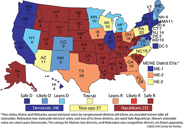
Figure 20.1: The electoral college map taken from UVA Center for Politics on 4/20/20
What do you observe from this map?
.
.
.
.
20.1.2 Modeling an Individual State
So, our first question is probably: how might we model who will win an individual state, say Florida and its 29 electoral votes?
To start, we’re going to assume that we can model each state with a single number, \(p\) which will represent the probability that a given state’s electoral college votes will go to the D or R candidate.
In fact, I’ll write this as \(p_i\) where the \(i\) is an index to the different states. This allows me to use the same notation for the different states we’re considering.
So, again, how might we get a reasonably accurate estimate of \(p_i\) for all the states (different \(i\)) of interest?
20.1.3 Interpreting Polling Data
We can go out and ask people. This is harder than it sounds.
- if we assume that everyone has already made up their minds, it is still not feasible to ask everyone. It’s too expensive absent of having the actual election.
- so instead, what we can do is take a sample of people and try to make an estimated guess about the larger population. This called statistical inference and we’ll do a lot of this in Winter Trimester.
- however, here, in doing our sampling, we might be concerned about bias in our results. Is our sample random enough that it adequately represents our population of interest?
- and what if everyone hasn’t made up their minds yet? Then, what do the answers represent?
- if we only sample a small portion of the population, it may also be because of randomness that we got unlucky, that we asked the wrong people. how do we account for the uncertainty that exists? Maybe, just by random chance our estimate isn’t that close to the true value.
- how do we interpret the difference between eligible voters, registered voters and likely voters?
This is complex, and for now, I don’t want to get too lost in the complexity. So, the main takeaway is be careful with the data you get. Make sure you understand what it means.
And in spite of all of these issues, there is usually not a lack of polling data. See:
But even still, interpreting these numbers can be challenging. Part of our challenge here is going to be finding accurate, reliable and meaningful data, and then figuring out exactly what to do with that data.
Let’s look at one example. Minnesota (MN) is a possible swing state, and a recent poll there shows Trump 44, Biden 49, or Biden +5. (https://www.realclearpolitics.com/epolls/latest_polls/elections/)
How do we interpret those numbers?
- What is our estimate of \(p\), again the probability of D winning the state?
- How do we model the other 7% of voters?
To use this data, we need to make some assumptions about things before proceeding down this path, and we’ll try to write down a model of what this represents. (Note: We’ll make and talk a lot about assumptions in Statistics this year and talk a lot about models.)
20.1.4 A Model of Voters
One approach we’ll use a lot in statistics this year is write down and use mathematical models to represent the real world.
Let’s let \(X\) be a random variable that represents the number of voters in MN that vote for the Democratic candidate, and let’s let \(n\) be the total number of actual voters. The D will win if \(\frac{X}{n} >0.5\).
What’s a random variable? For now, think about rolling a six-sided die. The outcome of a single roll is random. We don’t know the exact result until after we roll, but we know different possible outcomes before hand, and we can quantify how likely each is, i.e. their probabilities. For the dice case, assuming a fair die, each value between 1 and 6 is equally likely.
So again, in our voting case, \(X\), the number of votes the D gets, is our random variable. (As an aside, \(n\) is probably also a random variable.)
What we really want to know is \(P(\frac{X}{n} >0.5)\), which you read as “the probability that \(X\) over \(n\) is greater than 0.5”.
It turns out it’s not so straight forward to link our polling data \(p_i\) to what we actually want: \(Pr(X/n>0.50)\).
Part of the issue has to do with our model, and part of the issues has to do with uncertainty in our sampling results.
20.1.5 Linking Polling to Election Results?
In fact I’m not going to do this here except to quickly summarize why it’s difficult.
Polling data typically comes with a margin of error. This is one way we quantify the uncertainty in the data, and it depends on the number of samples we take (the number of people we poll). Quite simply, the more people we poll, the closer the our sample estimate is to the true value.
If we poll 1000 people, our margin of error is 3%. That means an estimate of 48% most likely lies between 45% and 51%.
Knowing this is useful, but again it complicates our analysis. Instead of just using our point estimate of the sample, a more thorough, complete, and detailed evaluation would also consider the impact of the uncertainty.
20.1.6 (Optional) Simulating an Election Outcome based on \(p\)
I will try to illustrate this challenge using simulation.
Let’s assume that:
- \(p=0.495\) (our estimate of how people will vote)
- \(X\sim Binom(n,p)\) (the distribution of votes, and its not a great assumption, but it’s easy to model!)
For the binomial model, think about counting the number of heads if we flip a coin 10 times. If we know the probability of a head on any individual coin toss (0.5), and we assume each toss is independent, then we can explicitly calculate the probability of seeing 6 head out of \(n=10\) flips (or whatever).
So, when actual the election happens, some number of voters go out and cast their vote. Well call that \(n\). (And for this exercise we’ll ignore third party candidates. Also, I’ll consider a “success” to be if an individual voter picks the Democratic candidate. )
Again, \(p\) represents the probability that each individual voter chooses the D candidate. (It’s more likely that most voters are fixed in their political affiliation, but let’s ignore that for now.)
Then, using the Binomial model, I can calculate the probability that a given number of \(n\) vote D. Or I can simulate using randomness, the number of \(X\), the number of people who vote for the Democratic candidate.
Remember, what we really want to know is \(P(\frac{X}{n} > 0.5)\), i.e. or in words, the probability that at least half the voters vote D.
Let’s examine a situation where \(\hat p= 0.49\). What is \(P(X/n > 0.5)\) for large \(n\)?
If we sample 1,000,000 (one million) people, the expected value will be 495,000 successes. But how often will there by at least 500,000 successes, when we consider the uncertainty?
Here’s a short chunk of R code that will allow us to simulate and plot these results:
## Simulate the # of D votes assuming 1,000,000 voters and p=0.49, and do this 1000 times
a <- rbinom(1000, 1000000, 0.495)

## create a histogram of the results
hist(a, breaks=15, main="Distribution of vote counts", ylab="count", xlab="# of D votes")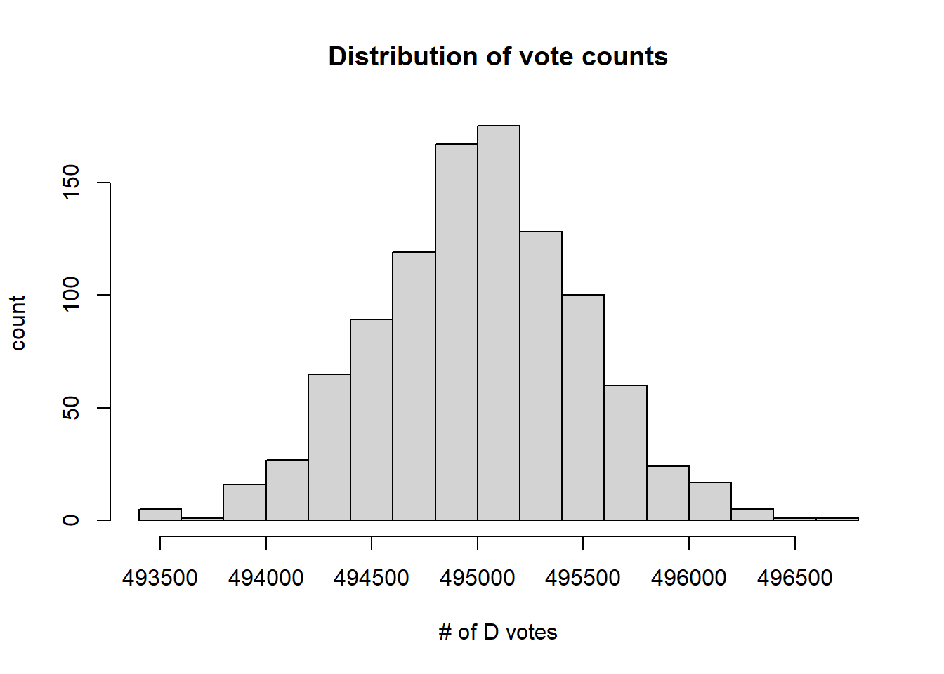
Figure 20.2: Simulated election results from a Binomial model with \(p=0.495\) and \(n=1000000\)
What do you notice?
This is a histogram and shows the distribution of results. We ran 1000 simulated elections. The x- axis is the # of votes that the Democratic candidate won in any given election, and the y- axis is the count of how many simulated elections they won that many votes.
This shows that all of the simulated outcomes result in between 493k and 497k D votes. In this case, assuming 1,000,000 total voters, then surprisingly, almost never does the D win the election in this state.
What’s happening here is correct. This distribution shows us the uncertainty in the results, but the uncertainty just isn’t that large.
And so, using the state level polling data may not be that helpful in this approach, mainly because if it’s below 50%, they lose and if it’s above 50%, they win.
So what could we do? I have two thoughts here:
- delve deeper into the meaning of the polling data and come up with a better model (i.e. improve on the assumptions from above), and/or
- simplify (at least to start) our approach of how we’ll model each state
20.1.7 A Simplified Approach
In the interest of time, I’m not (yet) going to go down that path of creating a better model of individual voters and tying that to the probability of a candidate winning the state. With statistical modeling (really all modeling), there are often multiple ways we might do something.
Note: Usually what I’ll do when my modeling gets complex, I try to bring myself back up to the 10,000 ft level to really make sure it’s clear what question I’m asking and that my approach makes sense and includes the right level of complexity.
Let’s look back at our map again:
Figure 20.3: The electoral college map taken from UVA Center for Politics on 4/20/20
Given that states are colored based on how likely it is they’ll vote a certain way, maybe we can ignore certain states and use the colors to guide our \(p_i\) values. In fact, we’ll ignore the individual voter entirely and just model the states.
Let’s consider only the “Leans” and “Toss-up” states as those that are “in play” (with their electoral votes):
- Leans D: NV(6), MN(10), MI(16), NH(4) - 36 total
- Toss-up: AZ(11), NC(15), NE-2(1), PA(20), WI(10) - 57 total
- Leans R: TX(38), GA(16), FL(29), OH(18), IA(6), ME-2(1) - 108 total
For a total of 201 electoral votes in play.
(And note, the above designations about which states are in which category aren’t universally agreed upon. More on that later.)
Without these states, D’s likely have 248-36 = 212 electoral votes and R’s likely have 233-108 = 125 electoral votes. Overall, the winner needs to get to 270, so in particular, D’s need to win 58 of the electoral votes from “in play” states whereas R’s need to win 145.
20.1.8 Guided Practice
Using the above projections and estimates, assume that D likely has 212 electoral votes locked up and R likely has 125 electoral votes locked up.
One (unlikely) path would be that the R wins all of the outstanding electoral votes and thus the election would end with the D getting 212 votes and the R getting 326 votes.
Find a path to victory:
- where the D barely wins and receives between 270 and 280 electoral votes
- where the R strongly wins and receives between 300 and 310 electoral votes
In each path be specific about which states are won and lost by each candidate. Based on the designation of your states, qualitatively, how likely do you think your calculated path is and why?
- how many possible paths are there? is each path equally likely? Why or why not?
20.1.9 Simplifying our Model
Let’s look at this map taken from: https://projects.economist.com/us-2020-forecast/president
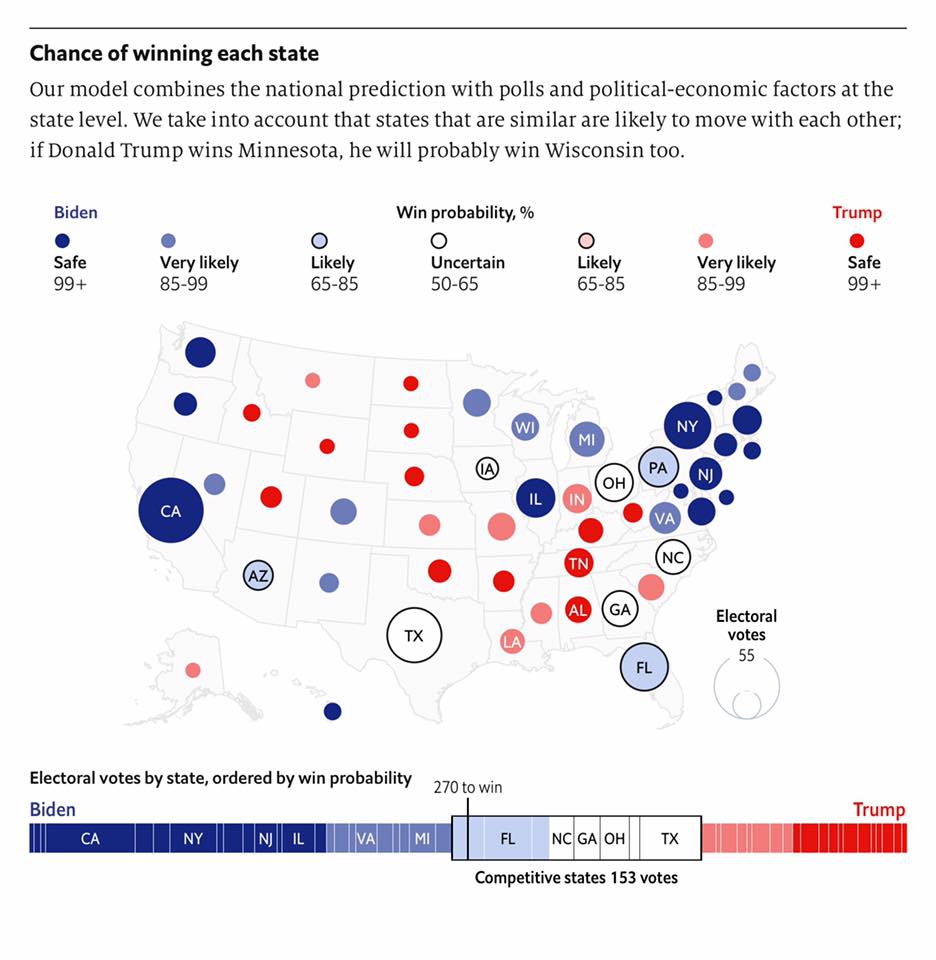
Figure 20.4: The electoral college map taken from The Economist from late July, 2020
(Which assigns slightly different values to some states.)
For simplicity, we can do something like:
- If it Lean’s D, there is a 75% chance D’s win
- If it’s a Toss-up, there’s a 50% chance D’s win
- If it Lean’s R, there is only a 25% chance D’s win
Where I’m ignoring the Safe and Very likely results and taking the middle of the Likely range and the bottom of the Uncertain range.
Here again, these are big assumptions that should be validated and/or further investigated after our initial pass model is complete.
Again, what I’m doing here is removing the discussion of the individual voters and instead just modeling \(P(S_i=D)\), the probability that a Democrat wins state, \(S_i\). Think of this like the probably that I flip a head.
20.1.10 Simulating Random Numbers
To use the above “chances” to model who wins which state, we’ll need to generate some random numbers.
Here’s a chunk of R code. One of the keys to this model is our use of the runif() function in R, which generates a continuous uniform random variable between 0 and 1, i.e. a random decimal value anywhere between 0 and 1 with equal probability.
Assuming there’s a 75% chance that D’s will win a certain state, here’s how I’ll model whether a D wins a simulated election in that state:
# simulate one value from a continuous uniform distribution and store it in the variable `a`
a <- runif(1)
# based on a, print out who won
if (a<0.75) cat("D won") else cat("R won")
## R wonNote: the blue-green lines with # are comments, for our benefit.
What this does is if our random number is between 0 and 0.75, we let the D win and if our random number is between 0.75 and 1, we let the R win.
Next, to simulate each state’s election, we’ll do this many, many times, and assuming the random number generator works correctly, a D should win in 75% of the random simulations.
To change the probability that a D wins, I just need to change the 0.75 value accordingly.
How would I change it if there was a 90% chance of the R winning?
20.2 Overview of the Model
So now that we can simulate a single state’s results, we can put this into a larger framework to simulate the overall election. Here’s my overview of what we’ll do:
Simulate a Single National Election:
- Generate a set of random numbers and use these to determine who wins each “in-play” state
- Based on who wins each state, assign the state’s electoral votes
- Sum up the total electoral votes won by each party across all states (to see who wins)
Simulate Many Elections:
- Run 10,000 (or so) simulated elections to evaluate the distribution (spread) of the possible results (think about a histogram)
- Calculate the proportion of the simulated elections where D’s win at least 58 electoral votes
Notes:
- In the first part that I need to generate the same number of random values as states that I’m simulating, so that the state results are independent.
- Only simulating a national election once may not tell me too much about the overall distribution depending on the variability of the results.
- If we simulate enough elections, it should create a distribution that accurately represents the true distribution
20.2.1 Coding this in R
Here’s a data frame I’ve put together which includes data for each of the 15 states that are “in-play”, including each state’s electoral college votes and the approximate probability that a D will win it based on the above assumptions.
my.state <- data.frame(
  abb=c("NV", "MN", "MI", "NH", "AZ", "NC", "NE", "PA", "WI", "TX", "GA", "FL", "OH", "IA", "ME"),
  votes=c(6,   10,   16,    4,   11,   15,    1,   20,   10,   38,   16,   29,   18,    6,    1),
  prob=c(0.75, 0.75, 0.75, 0.75, 0.5, 0.5,  0.5,  0.5,  0.5, 0.25, 0.25, 0.25, 0.25, 0.25, 0.25))
You will get very used to using data frames in R. For now, its a type of variable with columns and rows that’s quite flexible and very useful. Here’s what it looks like in R (and note there are 3 columns and 15 rows):
##    abb votes prob
## 1   NV     6 0.75
## 2   MN    10 0.75
## 3   MI    16 0.75
## 4   NH     4 0.75
## 5   AZ    11 0.50
## 6   NC    15 0.50
## 7   NE     1 0.50
## 8   PA    20 0.50
## 9   WI    10 0.50
## 10  TX    38 0.25
## 11  GA    16 0.25
## 12  FL    29 0.25
## 13  OH    18 0.25
## 14  IA     6 0.25
## 15  ME     1 0.25
20.2.2 Simulating an Single Election
Here is a custom function in R that goes through the steps to simulate one election. For now, focus more on the comments than the code.
sim.one <- function(verbose=F) {
  #1. simulate 15 different values between 0 and 1, one for each in play state
  a <- runif(15)

  #2. based on these and each state's prob, did D's win that particular state?
  # use vector math here to evaluate all states simultaneously.
  # won.each is a list of T/F values
  won.each <- a<my.state$prob

  # if the verbose parameter is true, print out the states that the D won
  if (verbose) {
    for (i in 1:15)
      if (won.each[i]) {cat(my.state$abb[i], " ")}
    cat("\n")
  }

  #3. if D's won, how many electoral votes did they win in that state?
  # votes.won is a list of electoral votes won, 0 if lost
  votes.won <- won.each*my.state$votes

  #4. so, how many electoral votes did the D win in total?
  total <- sum(votes.won)

  return(total)
}
sim.one(T)
## NV MN MI AZ NC NE TX ME## [1] 98This function returns how many of the in-play electoral votes the D won in this single simulated election, and if the verbose parameter is true, it also prints out the corresponding states in this path.
20.2.3 Simulate Many Elections and Examine the Distribution
Now, simulate 1000 elections so we can look at the distribution of outcomes:
# create storage for 1000 results
rslt <- vector("numeric", 1000)

# use a `for` loop to simulate how many votes the D got in the simulated elections
for (i in 1:length(rslt)) {
  rslt[i] <- sim.one()
}
And now we’ll use a “stripchart” (a type of histogram) to plot each result. Each point in the plot below is the result of one of our 1000 simulations, and the blue line is located at 58, the minimum number that the D need to win the presidency.
stripchart(rslt, method="stack", offset=0.4, at=0.15, pch=19, xlab="Number of Electoral Votes", ylab="Number of Simulations",
           main="Electoral votes won by D in in-play states")
abline(v=58, col="blue")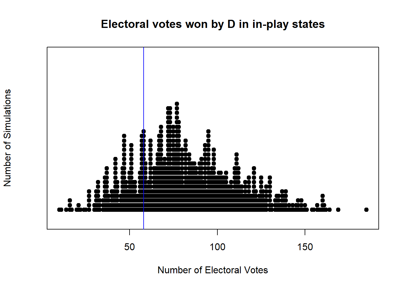
What do you observe?
.
.
.
To quantify the simulated probability, we’ll calculate the percentage of results where the D won at least 58 electoral votes as:
## [1] 0.792How should we interpret this number?
20.2.4 What’s Next?
First, is my model right? Almost certainly not. It’s based on a lot of assumptions that I don’t (yet) know if they are even close, including
- are the percentages of the individual states (including those I ignored) correct?
- are the various state’s results independent of one another?
- would modeling individual voters (including modeling eligible, registered and likely voters and different demographics) lead to a meaningfully different result?
Now that I have something working, I’d want to delve deeper into these questions to try to improve my model. And note, on the “is it right?” question, first, “No” its not, and second, we can revisit this in November to see how it did.
With most modeling efforts, it’s often less about building the model than it is about: “what can we use this model for?”
- Where might we spend resources (volunteering, donations, etc.) to impact the election?
- Based on this result, how much risk are you willing to take to make certain decisions about the future?
20.2.5 Useful Websites:
I can’t take credit for this approach. In particular, much of this is modeled after the following sites. And importantly, many of the following predictions or analysis are different than what we’ve shown above. And that’s ok! There’s often more than one way to approach these types of problems.
- https://projects.fivethirtyeight.com/2020-election-forecast/
- https://www.realclearpolitics.com/elections/2020/
- http://centerforpolitics.org/crystalball/2020-president/
- https://www.270towin.com/2020-election-forecast-predictions/
- https://cookpolitical.com/analysis/national/national-politics/latest-cook-political-report-electoral-college-map?
- https://fivethirtyeight.com/features/money-and-elections-a-complicated-love-story/
20.2.6 Guided Exercises: General Understanding
- Define a “random variable”. What is an example of a random variable we used above?
- Define a “distribution”. How is a distribution different from a histogram?
- Describe how we can use random values to represent and quantify uncertainty.
- What’s a place where there’s uncertainty in your life? Are you able to quantify that uncertainty?
20.2.7 Summary of what we did
This approach is generally known as Monte Carlo Analysis. It has applications in business analysis, risk management and more.
We start with a static (fixed) model of how things work, with inputs and outputs, and then we add uncertainty to the inputs to understand and evaluate the uncertainty that results in our outputs.
In this case our inputs were who wins each state and the output is who wins the election.
Overall, what we did was:
- A quick intro to electoral politics
- How might we model the outcome of an individual state?
- how good is our data and what does it mean?
- simplifying our process
- Compiling the state results
- Simulating many, many elections
- How should we interpret the results? and next steps.
- Other applications of Monte Carlo Analysis
20.3 Simulating Stock Market Returns
How might we model and simulate stock market returns? How do different types of assets perform? What is the advantage of a diversified portfolio? These are the types of questions we’ll attempt to answer.
Let’s suppose we had three asset classes to choose from. Each has a mean and std deviation of return.
Imagine we have different investable assets - might be different stocks themselves or might be different asset classes (e.g. large cap vs. REIT vs bonds). What are the expected returns and variance of each? What do these returns and risks mean about long term value? We could simulate this.
assets <- data.frame(return=c(0.08, 0.05, 0.02), risk=c(0.1, 0.02, 0.01))
row.names(assets) <- c("A", "B", "C")
assets
## return risk
## A 0.08 0.10
## B 0.05 0.02
## C 0.02 0.0120.4 Part 1: Simulating a Single Asset
Let’s look at a single asset, in this case one where the mean return is 8% and the standard deviation of the return is 10%.
We think of returns on an asset are a percentage. If you start with an investment of /$100 and after 1 year you have $105, then you’ve earned a 5% return. (The change divided by the original amount.)
## [1] 0.05Returns aren’t fixed, and there is risk associated with them. We’ll model risk as a return being a random variable with a mean result AND a standard deviation. So, in any given year the returns for that asset would have a distribution associated with it:
sim.return <- function(mean, stdev)
{
  for (i in 1:1000) {
    a <- rnorm(1000, mean, stdev)
  }
  hist(a, main="distribution of annual returns")
}
sim.return(0.08, 0.10)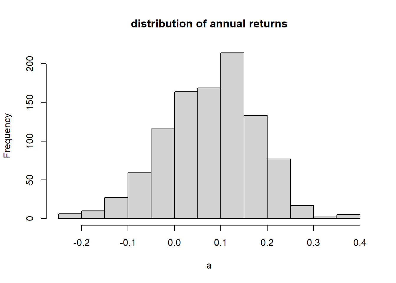
Here we’ve simulated this as having a Normal distribution, which is close enough for our purposes here. (In fact actual returns typically have heavier tails than a Normal distribution would allow.)
Of course, these returns accumulate over time (assuming you hold/don’t sell the asset). So if year 1 had a 4.8% return, year 2 had a -0.8% return and year 3 had a 6.1% return, overall, the return would be:
## [1] 1.103033Equal to a net return of 10.3%.
Note, we don’t add these returns together or even average them. Instead, to calculate the overall return, we need to add one (1) to each year’s return, multiply the consecutive returns, and then subtract one (1) from the overall result.
It can be informative to graph these cumulative returns over time, say 25 years:
a <- vector("numeric", 25)
a[1] <- 1
r <- rnorm(25, 0.08, 0.10)
for (i in 2:25) {
  a[i] <- a[i-1]*(1+r[i])
}
plot(a, xlab="year", ylab="cumulative value", main="simulated return",
     type="b", ylim=c(0, max(a)), col="darkblue")
abline(h=1, col="red", lty=2)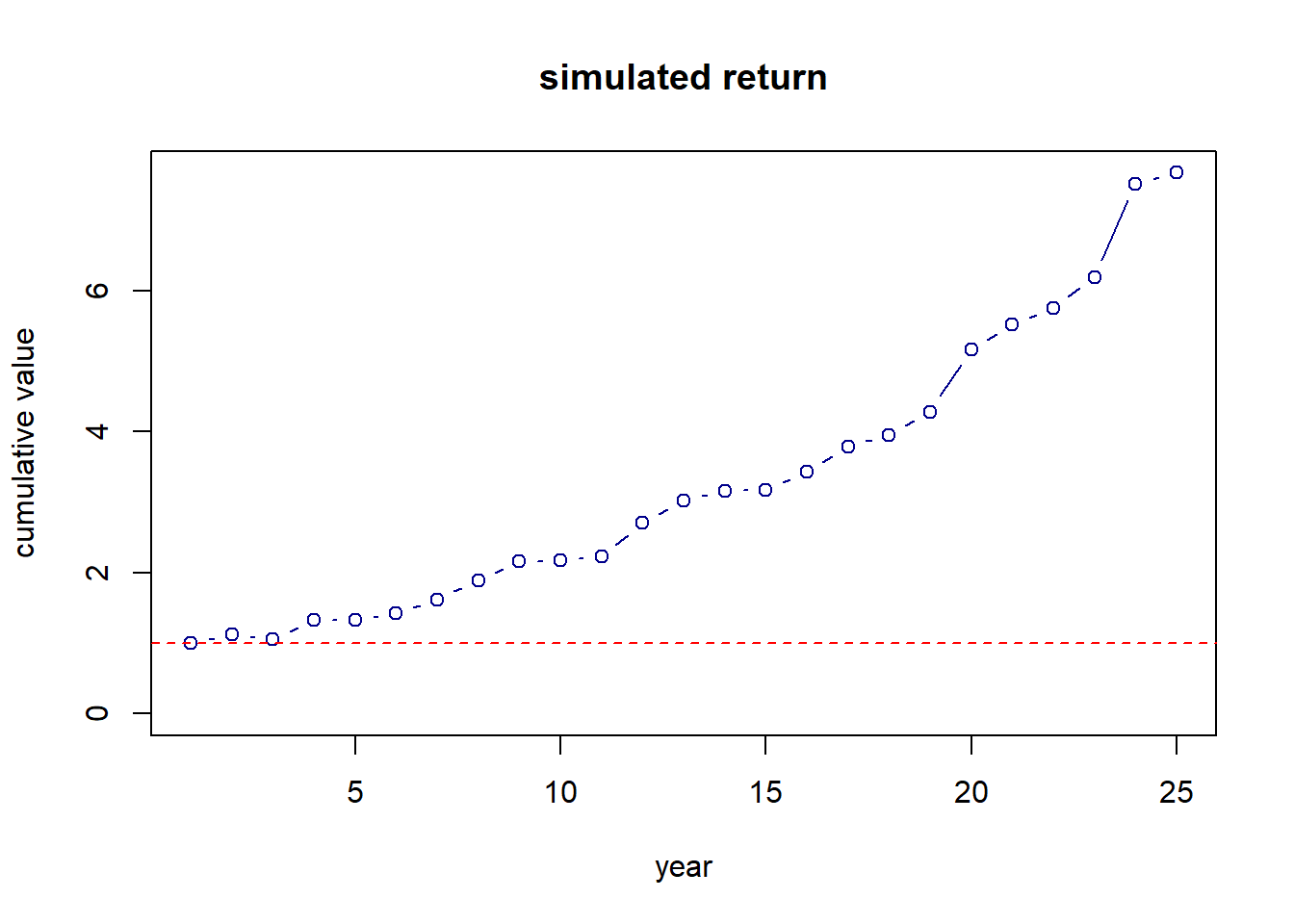
Here we see the cumulative nature of returns. Generally, even with a lot of variability, if the mean return of an asset is positive, time invested will lead to growth.
This graph is interesting, but since it’s based on a set of random values, we’ll see a lot of variability each time we run this function. One simulation doesn’t tell us very much. Instead, we’re probably more interested in the distribution of results we might see over time.
Here is a function that simulates many, many different returns over 25 years and then displays the 95% range of results each year:
sim.years <- function(mean, stdev) {

  nsim <- 250                           # The number of different simulations
  val <- matrix(nrow=nsim, ncol=25)     # Storage for the results

  for (j in 1:nsim) {
    val[j, 1] <- 1
    b <- rnorm(25, mean, stdev)           # Simulate the random results
    for (i in 2:25) {
      val[j, i] <- val[j, i-1]*(1+b[i])   # Calculate the cumulative returns
    }
  }

  upper <- apply(val, 2, quantile, 0.975)   # Determine the upper interval
  lower <- apply(val, 2, quantile, 0.025)   # Determine the lower interval
  average <- apply(val, 2, mean)            # Determine the average result

  plot(1:25, upper, type="l", ylim=c(min(lower), max(upper)), lty=2,
       ylab="Returns", xlab="Years", main="95% range of simulated returns")
  lines(1:25, lower, lty=2)
  lines(1:25, average)
  abline(h=1, col="red", lty=4)
}

sim.years(0.08, 0.10)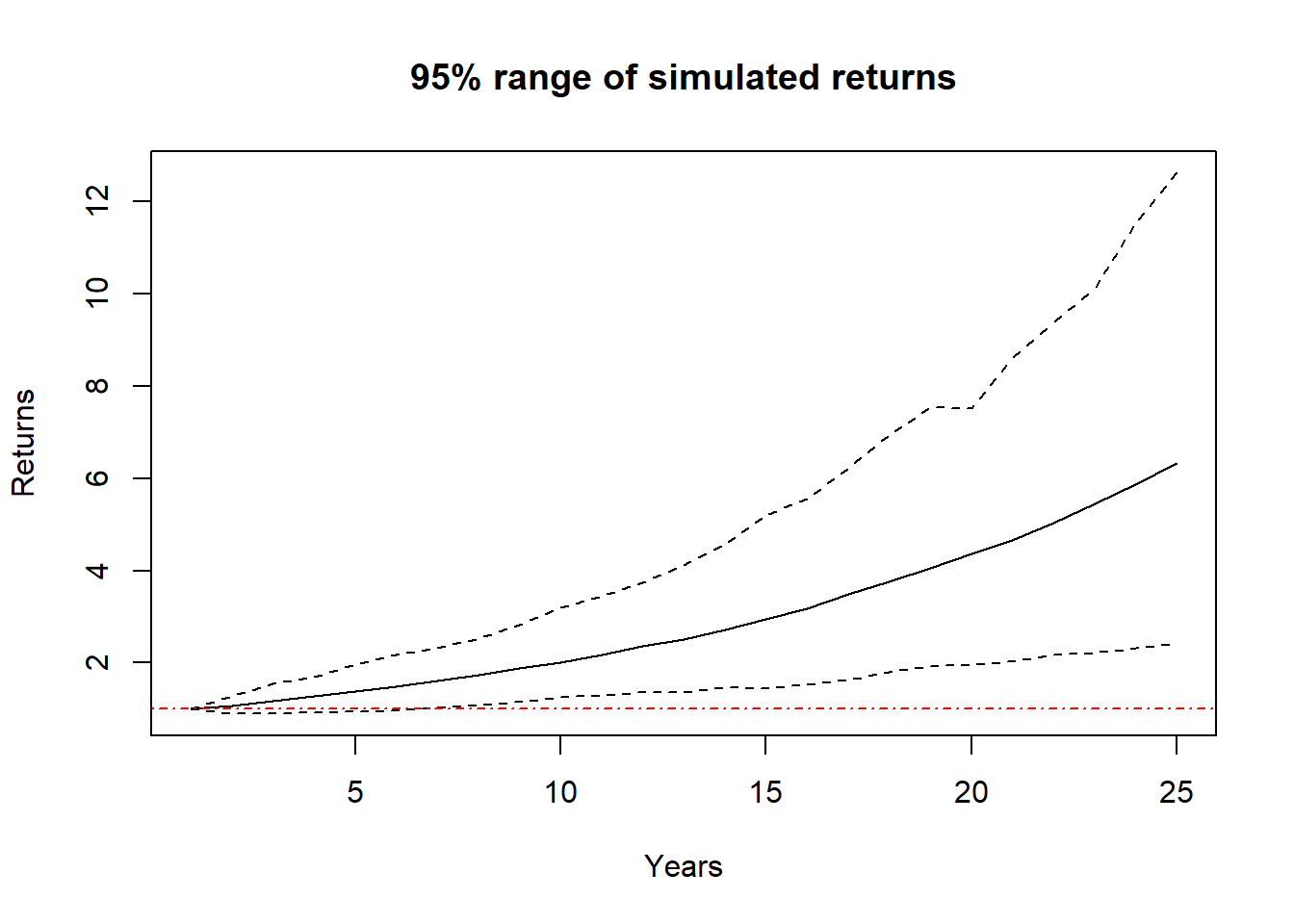
In this graph, the dark blue dashed lines are the ranges of the middle 95% of results, the black line is the average result, and the red dashed horizontal line indicates where we started.
Again, this cumulative nature of growth is shown. We do see in early years there is a reasonable chance of loss, however, over the full time of the simulation, we see a range of outcome that all show growth.
20.4.1 Are Returns and Standard Deviations Constant?
Suffice it to say that these returns depend a lot on the values of the mean and standard deviation. For example:
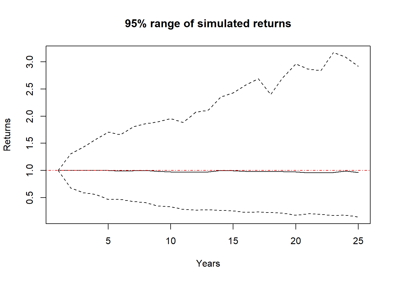
Different asset classes typically have are different return/risk profiles. Large cap stocks have higher returns, and higher risks. Bonds (or US Treasury Notes) typically have lower returns and very little risk. And, note there are a number of ways we might characterize “risk” for investments, and standard deviation is a good start.
Here it’s probably worth exploring Bull vs. Bear market and how the relationship between mean and standard deviation impact these results…
20.5 Part 2: Examining Correlation Between Assets
Let’s play with some stock data from Apple and Alaska Airlines, downloaded from Nasdaq.com
Here is a plot of both stocks:
plot(as.Date(stocks$Date, "%m/%d/%Y"), stocks$AAPL, type="l", col="darkblue", ylim=c(0, 175), ylab="Price", xlab="Date")
lines(as.Date(stocks$Date, "%m/%d/%Y"), stocks$ALK, col="red")
legend("topleft", legend=c("AAPL", "ALK"), lty=1, col=c("darkblue", "red"))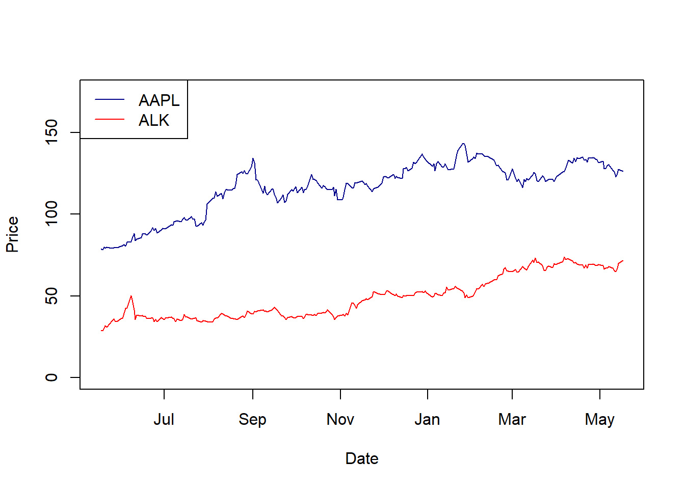
Calculate the return and standard deviation of each?
Since these are time series, we need to subtract and divide:
calc.returns <- function(ts) {
  a <- vector("numeric", length(ts)-1)

  # NOTE: the data is backwards in time (latest dates are first)
  for (i in 1:(length(ts)-1)) {
    a[i] <- (ts[i]-ts[i+1])/ts[i+1]
  }
  # `a` now contains the set of daily returns.
  cat("mean", mean(a), "stdev", sd(a), "\n")
}
calc.returns(stocks$AAPL)
## mean 0.002128682 stdev 0.02221801## mean 0.004244958 stdev 0.03625696## Be careful about whether to use the geometric vs. mean as the average
## I think if we want our standard deviation, we need to use the mean?And note these are daily returns. How would we convert these to annual returns?
We also might look at the correlation between these two assets. First let’s plot the relationship:
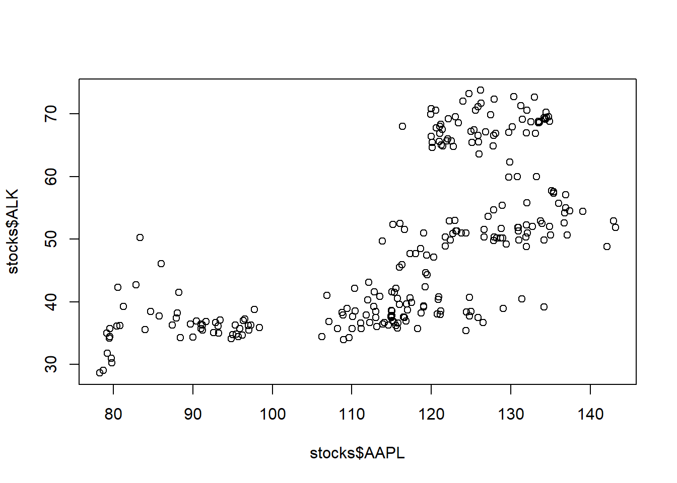
And then calculate the correlation itself:
## [1] 0.6499815Generally what this shows is that these two assets vary (roughly) together.
20.6 Part 3: How and Why Should We Build a Diversified Portfolio?
How should we allocate our funds, assuming different levels of correlation? Again, we could simulate this.
When we think about having a diversified portfolio we want to account for “bad” years. If assets are highly correlated, in a bad year we lose value on both, which is not desirable.
When simulating, we need to force good and bad years, instead these should come out of the simulation itself - we’ll simulate correlated data, and good and bad results will naturally occur.
Overall, the here approach will be to simulate highly correlated assets and then weakly correlated assets, and compare the results.
20.6.2 Comparing Portfolios with Different Correlations
Let’s just look at two different cases: (i) highly correlated assets vs. (ii) weakly correlated assets.
# set the return and covariance matrix variable
r1 <- list(mu=c(0.08, 0.05, 0.02),
                sd=c(0.10, 0.04, 0.01),
                r=matrix(c(1, 0.7, 0.7, 0.7, 1, 0.7, 0.7, 0.7, 1), 3,3))

r2 <- list(mu=c(0.08, 0.05, 0.02),
                sd=c(0.10, 0.04, 0.01),
r=matrix(c(1, 0.2, 0.2, 0.2, 1, 0.2, 0.2, 0.2, 1), 3,3))## mean total return: 3.19
## sd total return: 0.7## mean total return: 3.21
## sd total return: 0.58The brilliance of this approach is that for the same expected return, by choosing uncorrelated assets, we’ve been able to reduce our risk!
20.6.3 For More Research
- How to convert the daily returns/ and standard deviation into annual values?
- What do we mean by risk/reward profile?
- Have students build their own portfolios?
- How does adjusting the asset allocation change expected returns and standard deviations?