Chapter 16 $\chi^2$ and Goodness of Fit Tests

16.1 Overview

A few chapters ago we looked at hypothesis testing and inference for count and proportion data, where we both compared one sample to a prior estimate and we also compared two samples to each other. In this chapter, we will come back to count and proportion data, expanding our repertoire to allow for additional comparisons.

We will start by examining so called “one-way tests”, where we look at data with more than two categories and asking if the counts are basically equivalent, $p_1=p_2=p_3$ (i.e. tests of homogeneity or uniformity.) We will then expand that to evaluate if a set of data with more than two categories comes from a distribution with suspected (hypothesized) non uniform prior probabilities (i.e. goodness of fit tests).

After that, we will further expand this approach to look at additional variables in two-way tests and be able to answer questions about whether multiple categorical variables exhibit independence.

16.1.1 Learning Objectives

By the end of this chapter, students should be able to:

Describe the form of the $\chi^2$ distribution and explain how to determine the appropriate degrees of freedom
Write an appropriate null and alternative hypothesis for a given test and correctly interpret the results in context
Determine the expected values of counts under different null hypothesis
Explain the form of our goodness of fit test statistic and calculate it for a given set of observed and expected counts
Perform a one-way $\chi^2$ test for homogeneity
Perform a one-way goodness of fit test
Perform a two-way $\chi^2$ test for independence
Discuss what steps we can take after we reject $H_O$

16.2 One-way $\chi^2$ Test for Homogeneity (i.e. Equal Proportions)

The first type of test we will run describe is used to evaluate if observed counts from different categories could have reasonably come from a true distribution where each category was equally likely.

As an example, a typical Skittle bag contains 56 pieces, and there are 5 colors: Purple, Green, Yellow, Orange and Red. Let’s suppose we open a bag and find the following counts:

color	count
Purple	12
Green	7
Yellow	4
Orange	16
Red	17

These counts aren’t all equal, but we might ask, is it reasonable that our observed counts come from a “true” distribution where all colors are equally represented? Maybe all Skittles of each color in equal proportions are first poured into a huge bowl, mixed, and then 56 candies (or so) are chosen at random to fill an individual bag. As such, is any difference between what we observe and what we “expect” purely based on random chance?

What we’re really asking here is how good of a fit is a distribution where all proportions are the same. In fact, that will be our null hypothesis, namely $H_0: p_P = p_G = p_Y = p_O = p_R$, where the subscripts represent the different colors. Our alternative hypothesis will be that at least one proportion is different. (Note: This is a different formulation of our alternative hypothesis. As we’ll see, all we can do at this stage is reject the idea that all proportions are equal. We will use a different method to see which proportion or category that might be.)

Now, to test this null hypothesis, our general approach will follow the same steps as we previously did for hypothesis testing, namely:

Figure out the null distribution and form of our test statistic
Determine the critical value based on our $\alpha$ level (note there is usually only one)
Collect the data and calculate the test statistic
Compare the test statistic to the critical value
Calculate the p-value of our test statistic under the null hypothesis
Make our conclusion

Although the process is the same, quite a bit of the detail is new here.

16.2.1 The Form of our Test Statistic

Before considering our null distribution, we should first discuss our test statistic, which also has a new form. Remember, the null distribution is the distribution of the test statistic if the null hypothesis is true. So, starting with the test statistic makes sense.

We first need to consider the expected results if the null hypothesis of equal proportions is true. If so, we’d expect (on average) $56/5=11.2$ candies of each color in the bag. (As we saw in an early chapter, an expected value does not have to be a count that can actually occur!)

Here is our above table with the expected results under $H_0$, along with the observed results.

color	expected result	observed count
Purple	11.2	12
Green	11.2	7
Yellow	11.2	4
Orange	11.2	16
Red	11.2	17

Of course both the expected and observed counts sum to 56.

We now want a test statistic that characterizes how far away the observed results are from the expected results.

How big of a difference is there? Let’s do some analysis in R. In the code chunk below I have created vectors containing the expected and observed counts.

obsvd <- c(12, 7, 4, 16, 17)
expct <- rep(56/5, 5)

We might start by thinking we should just calculate the sum of the differences. Let’s attempt this. First we’ll create a vector of the differences between expected and observed for each color:

obsvd-expct

## [1]  0.8 -4.2 -7.2  4.8  5.8

And now we’ll sum this vector:

sum(obsvd-expct)

## [1] 3.552714e-15

What do you observe? (In fact, I don’t know why R doesn’t think this is exactly 0? Regardless, it3.55e-15` is a very small number.)

Importantly, for any set of observed and expected values, the sum of the differences will be exactly 0. So, this idea of just subtracting won’t work.

So what next? We might consider using the mean (which will also be zero!), the sum of the absolute value (which is less mathematically tractable) or the sum of squared differences. It’s this last idea that we’ll pursue.

Specifically, for our test statistic we’ll use the following form, and hopefully you recognize how this is a measure of how far away our observed counts are from the expected results:

\[\chi^2 = \sum \frac{(observed-expected)^2}{expected}\]

Why do we scale by the expected value? In short, that allows us to compare ANY data to the null distribution, regardless of its magnitude.

Continuing with our Skittles example, using this formula we find our test statistic as follows. First note that by squaring the differences, all the values become positive:

(obsvd-expct)^2

## [1]  0.64 17.64 51.84 23.04 33.64

Hence our actual test statistic is:

sum((obsvd-expct)^2/expct)

## [1] 11.32143

This R calculation is equivalent to calculating this value for every cell and summing them together, as: \[\frac{(12-11.2)^2}{11.2} + \frac{(7-11.2)^2}{11.2} + \frac{(4-11.2)^2}{11.2} + \frac{(16-11.2)^2}{11.2} + \frac{(17-11.2)^2}{11.2} = 11.32\]

At a minimum, I would hope you recognize that as the observed counts get further away from the expected values, this number will grow, and in particular it accounts for larger deviations (because of the squaring) more than smaller ones.

16.2.2 The Null Distribution

So now that we know our test statistic, what is it’s distribution? For goodness of fit and $\chi^2$ testing we will use what is known as a $\chi^2$ (“chi-squared”) distribution. This will again incorporate the idea of degrees of freedom, which in this case will be the number of categories -1. So, for our Skittle example, there are 5 categories (i.e. 5 different colors), so we have 4 degrees of freedom. As mentioned above, since we scale the test statistic, the only information we need for our null distribution is the degrees of freedom.

Here is what a $\chi^2$ distribution looks like with 4 degrees of freedom:

x <- seq(from=0, to =10, by=0.01)
y <- dchisq(x, 4)
plot(x, y, type="l", ylab="probability")

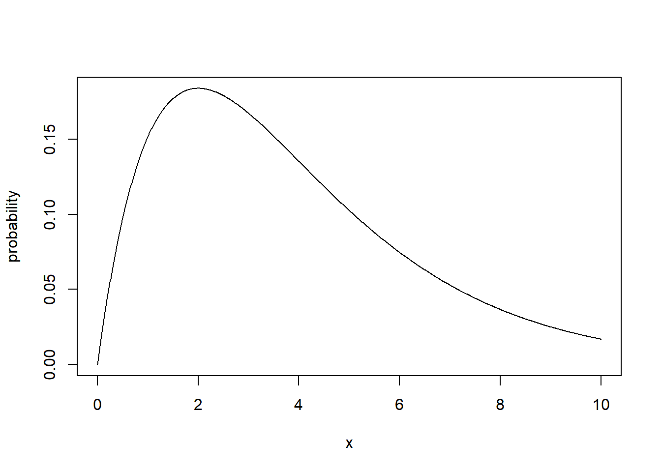
Which has a different shape than what we’re used to! Note that this is still a probability distribution, similar to the Normal or t-distribution. (i.e. it “sums” to one, it describes all possible outcomes, etc.)

Luckily, as with all of the other distributions we’ve seen, R makes the following functions available:

dchisq(): the density (height) function at a particular value of $x$
pchisq(): the probability of a random value less than $x$
qchisq(): the $x$ value associated with a specific cumulative probability
rchisq(): generate random variables from the distribution.

Technically a $\chi^2$ distribution is the sum of squares of independent Normal distributions. That’s a mouthful, and maybe simply worth knowing that this is similar to the square of a Normal distribution. What this means is that all $x$ values are positive and it is NOT symmetrical.

16.2.3 Guided Practice

Simulate many bags of Skittles example assuming equal proportions in the population using sample(), and for each bag calculate the corresponding test statistic. Next, create a histogram of the distribution of test statistics, making sure to set freq=F. Using dchisq(), overlay the null distribution on your plot. What do you observe?

16.2.4 Finding our Critical Values

You may have observed in the above distribution that there were no negative values. In fact, with this form of a test statistic, a perfect fit (i.e. observed counts = expected counts) would have a value of exactly zero, and any deviation from perfect yields a larger test statistic value.

An important implication of this is that we will only reject $H_0$ if our test statistic is too big. Because of this, all $\chi^2$ goodness of fit tests are one-sided and we’ll only need to find the upper critical value.

Hence to find our critical value for the Skittles example we’ll use

qchisq(0.95, 4)

## [1] 9.487729

For $\alpha=0.05$, this function calculates the value of the $\chi^2$ distribution (with $df=4$) that 95% of the probability is below.

16.2.5 Comparing our Test Statistic to the Critical Value

Based on our calculated test statistic, $\chi^2 = 11.32$, we can see that we will reject $H_0$.

Here is a plot of the null distribution and test statistic just to reinforce the point:

x <- seq(from=0, to =12, by=0.01)
y <- dchisq(x, 4)
plot(x, y, type="l", ylab="probability")
abline(v=qchisq(0.95, 4), col="red")
abline(v=11.32, col="darkgreen")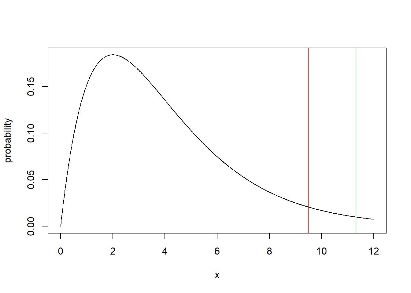

The test statistic is outside the upper critical value.

16.2.6 Calculating p-values

Similar to how we did this previously, here we’ll find our p-value as:

pchisq(11.32, 4, lower.tail=F)

## [1] 0.02319356

Again since we are only running one-sided tests where we reject only if our test statistic is too big, we will always use lower.tail=F here.

Finally, we will interpret the p-value as we always have. In this case, since the p-value, $p=0.023$ is less than $\alpha=0.05$, we will reject $H_0$ and conclude at least one of the probabilities of colored candies is different.

16.2.7 Necessary Conditions of Goodness of Fit Testing

It is important to recognize that to use a $\chi^2$ distribution and draw the conclusions we do from it, there are a few necessary conditions that must be met. These include:

Our data come from a simple random sample,
The sample is less than 10% of the population,
The expected values of all cells should be $\ge 5$.

16.2.8 Using R Functions for One-way Goodness of Fit testing

As we previously saw with t- tests and two sample testing, R has a number built-in functions to make hypothesis testing easier by handling many of the low level details. This is also true perform goodness of fit testing, and to do this we’ll use the chisq.test() function.

For our previous Skittles example where we tested homogeneity, we’d use:

chisq.test(c(12, 7, 4, 16, 17))

## 
##  Chi-squared test for given probabilities
## 
## data:  c(12, 7, 4, 16, 17)
## X-squared = 11.321, df = 4, p-value = 0.02318

Note that these results are the same as we found above doing this by hand! The X-squared result is our test statistic and (obviously) the p-value is our p-value.

16.2.9 Guided Practice

Does EPS gear (hoodies, shirts, bags) sell equally well among each class and faculty? The following table shows recent sales in units to each group.

Middle schoolers	Freshman	Sophomores	Juniors	Seniors	Faculty
51	35	40	60	52	48

What are the total sales (in units)? If sales were equally distributed among groups, how many items would be expected in each group?
What are your null and alternative hypothesis?
What is your null distribution? How many degrees of freedom are there?
What is the critical value at $\alpha=0.05$?
Create R vectors of both the observed and expected counts. What is your test statistic?
What is the p-value, and what do you conclude?
Use the chisq.test() function to confirm your results.

16.2.10 Optional: Simulating the Null Distribution

Above we jumped straight to the idea that our null distribution was chi-squared with 4 degrees of freedom. We could alternatively use simulation to build our null distribution without relying on such statistical theory. As we’ll see, the shape of the resulting distribution is quite similar.

As a reminder, the null distribution is the probability distribution of the test statistic if the null hypothesis is true. What is our null hypothesis here? That all colors occur in equal proportions. So, we’ll use simulation to build the distribution of test statistics, if that’s true.

The following code creates a null distribution under the assumption of equal distribution of colors. It uses the sample function to create a simulated Skittles bag, and then calculates the the test statistic for that bag. It then repeats this process 10,000 times to evaluate the full distribution of possible test statistic values, again assuming our null hypothesis is true.

# what are the possible colors of candies
a <- c("R", "Y", "O", "G", "P")

# expected results if all colors are evenly distributed
exp <- rep(56/5, 5)

# storage for simulated results 
obs <- vector("numeric", 5)
dist <- vector("numeric", 10000)

# main simulation loop
for (j in 1:10000) {
  # create one bag of skittles with 56 candies, 
  #  each color sampled with equal probability
  bag <- sample(a, 56, replace=T)

  # find the count of the colors in the bag
  for (i in 1:5) {
    obs[i] <- length(which(bag==a[i]))
  }

  # calculate and store the test store the test statistic for our bag
  dist[j] <- sum((obs-exp)^2/exp)
}

# plot the histogram and our original findings
hist(dist, breaks=25, main="null distribution")
abline(v=11.32, col="red")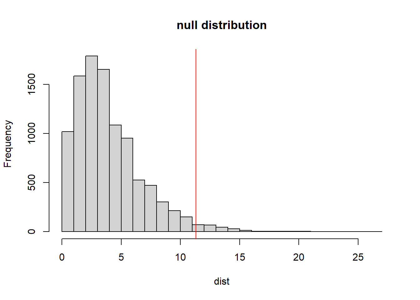

The red vertical line shows the observed test statistic from our original bag. As shown, that value is quite unlikely if the null hypothesis is true.

Below is the same distribution, this time plotted as density, and showing the chi-squared distribution with 4 degrees of freedom in blue. Note the strong similarities.

hist(dist, breaks=25, main="null distribution", freq=F)
x <- seq(from=0, to=25, by=0.1)
y <- dchisq(x, 4)
lines(x,y, col="blue1")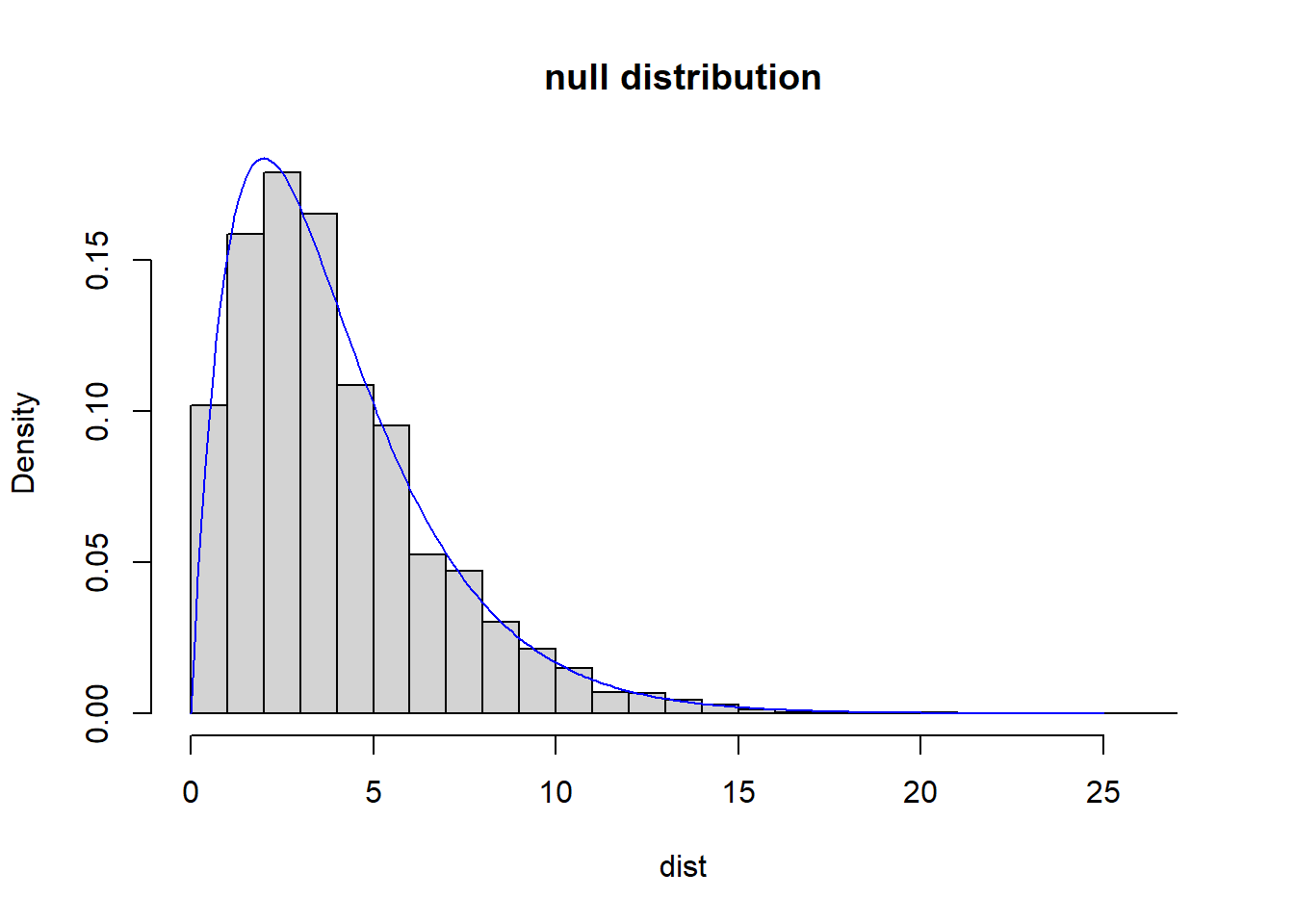

The intent of showing this is for you to see directly that the null distribution based only (i) on simulated values where we know that the true proportions of the different colors is the same as (ii) a $\chi^2$ distribution with 4 degrees of freedom.

16.3 One-way Goodness of Fit Testing

In the previous section we learned about using $\chi^2$ testing to evaluate (using a hypothesis test) if the observed proportions (counts) of multiple groups can reasonably be considered the same. Here, we’ll employ the same general approach, but ask a slightly different question. Instead of all proportions being equal, we might have a case where prior estimates of each proportion are known, and we want to test if observed counts follow those proportions. In other words, we have some prior “distribution” in mind (other than uniform), and we want to see if our data is a good fit.

For example, imagine the following data describing the observed representation of different races on juries, compared to their proportions in the community (taken from os4 page 229):

Race	White	Black	Hispanic	Other	Total
Representation on Juries	205	26	25	19	275
% of Registered Voters	0.72	0.07	0.12	0.09	1.00

Based on this data, our question is: “Is it reasonable to assume that the representation on juries matches the overall diversity of the population?” (i.e. Is the observed variation simply the result of random sampling, OR is there possibly some bias in jury selection?)

(Note we have both counts and proportions in this data, and hopefully you’ll see that they’re basically interchangeable, at least conceptually. However for this goodness of fit testing, we’ll always use counts.)

How would we test this?

Think back to our previous framework. To answer our question we’re going to:

Figure out the null distribution that would exist if the representation on juries matched the percentage of registered voters.
Create a test statistic that represents how far away our observed data are to the expected results (if the null hypothesis were true), and then
Compare our test statistic to our null distribution, and use this to quantify about how likely our test statistic is if the null hypothesis is true (i.e. our p-value).

By now, this approach should sound pretty familiar. The main differences between this test and the previous test of homogeneity are (i) how we write our null hypothesis and (ii) how we calculate the expected counts.

16.3.1 Our Null Hypothesis

The null and alternative hypothesis are a bit more difficult to write for these types of tests, and we really need to consider what “randomness” means here.

Our null and alternative hypothesis will be:

$H_0$: The jurors are a “random” sample based on the % of registered voters. In other words, there is no racial bias in who serves on a jury, and the observed counts reflect natural sampling fluctuation.

$H_A$: The jurors are not randomly sampled, i.e. there is some racial bias in juror selection. The probability of the differences between the observed and expected counts is just too unlikely.

As you see, I’m less likely to write this with the parameter values themselves, and more likely to describe this qualitatively.

Because of randomness, even if $H_0$ is true, the observed and expected counts will rarely perfectly match. However, the observed proportions should roughly match the expected probabilities.

One other important note: “random” does NOT necessarily mean “uniform”. Random observations can come from ANY underlying distribution.

16.3.2 The Null Distrtibution and Critical Value

Remember that the null distribution describes the possible values of the test statistic we’d expect to see (and how likely they are) if the null hypothesis is true.

As we did with our Skittles test, we’re going to use what’s known as a $\chi^2$ distribution, in this case, since there are $n=4$ groups, we’ll have $df= n-1=3$ degrees of freedom.

Why is it that we can use the same null distribution? Because we are scaling each category by its expected value.

So, how do we find our critical values? The critical value defines the threshold for which we deem an observed test statistic to be too unlikely. Again, since we only reject if our test statistic is too big, there is only one critical value.

And just like we’ve done previously, we can use the qchisq() function to find our critical value. Given we have $df=3$, at $\alpha = 0.05$ we’d have:

qchisq(0.95, 3)

## [1] 7.814728

Hence we will reject $H_0$ if our test statistic is greater than $7.815$.

16.3.3 Calculating the Expected Counts

Calculating the test statistic proceeds almost identically to our previous approach, with the main difference being how we determine the expected counts.

Assuming we start with expected proportions, we can simply multiply these proportions by the total (observed) count to find the expected counts.

So in this example, I will simply multiply the total number of jurors (275) by their respective percentage of the electorate. This yields the following results:

Race	White	Black	Hispanic	Other	Total
Observed Representation on Juries	205	26	25	19	275
% of Registered Voters	0.72	0.07	0.12	0.09	1.00
Expected Count (under $H_0$)	198	19.25	33	24.75	275

where 72% of 275 = 198, 7% of 275 is 19.25, etc., etc.

Importantly, these expected counts represent the number of jurors we’d expect to see if they were selected exactly in accordance with the % of registered voters. (If $H_0$ were true.) It has nothing to do with observed counts, except that it uses the total.

Note that if we have our percentages in an R vector, we can figure out expected counts as:

prop <- c(0.72, 0.07, 0.12, 0.09)
prop*275

## [1] 198.00  19.25  33.00  24.75

Also remember that if you don’t easily have the row totals, we can find find this using the sum() function.

16.3.4 Our Test Statistic

As above, we want our test statistic to reflect how far away our observed counts are from the expected results. We’ll use the exact same form as above, namely:

\[\chi^2 = \sum \frac{(observed-expected)^2}{expected}\] For our data, this is:

\[(205-198)^2/198 + (26-19.25)^2/19.25 + (25-33)^2/33 + (19-24.75)^2/24.75 = 5.89\]

In R, we would perform this calculation as:

## Vector of observed counts
o <- c(205, 26, 25, 19)
## Vector of expected counts
e <- c(198, 19.25, 33, 24.75)

## Find the test statistic
ts <- sum((o-e)^2/e) 
cat("test statistic:", round(ts,3), "\n")

## test statistic: 5.89

To remind you of what was discussed above about test statistics:

As the observed counts get further away from the expected counts, our test statistic will get bigger.
By dividing/scaling by the expected counts, we are ‘standardizing’ this result to enable comparison against the appropriate $\chi^2$ distribution.

16.3.5 Evaluating the Test Statistic

Above we found our critical value to be $7.815$. Given the test statistic of $5.89$, we will fail to reject $H_0$.

16.3.6 Calculating the p-value

In this case, particularly since our test statistic is below the critical value, we don’t need to calculate the p-value, but let’s do it anyways:

pchisq(5.89, 3, lower.tail=F)

## [1] 0.1170863

As a reminder, for $\chi^2$ testing, we’ll always use lower.tail=F

Hence, based on this data, we fail to reject $H_0$ and conclude there is no statistically significant difference between proportion different races serve on juries and their proportion in the overall population.

16.3.7 Using R Functions for One-way Goodness of Fit testing

Again here we can use the chisq.test() function to run a goodness of fit test, with a slight modification.

To test the non-equal proportions (i.e. one way goodness of fit testing), such as in our jury selection example we need to include a second parameter, p which gives the expected proportions as:

chisq.test(c(205, 26, 25, 19), p=c(0.72, 0.07, 0.12, 0.09))

## 
##  Chi-squared test for given probabilities
## 
## data:  c(205, 26, 25, 19)
## X-squared = 5.8896, df = 3, p-value = 0.1171

which again, matches the results we found above when doing the analysis by hand.

16.3.8 Guided Practice

A 2017 survey looked at different companies share of the sneaker market and calculated the following percentages: Nike (35.6%), Jordan (15.7%), Adidas (11.4%), Sketchers (4.7%), New Balance (3.5%), Converse (3.5%) Under Armour (2.5%), Other (23.1%)

You survey 150 teenagers about the brand of shoe they were wearing and found the following results:

Brand	Count
Nike	61
Jordan	20
Adidas	15
Sketchers	10
New Balance	2
Converse	12
Under Armor	0
Other	30

props <- c(0.356, 0.157, 0.114, 0.047, 0.035, 0.035, 0.025, 0.231)
shoe_counts <- c(61, 20, 15, 10, 2, 12, 0, 30)

Is it reasonable to assume that your sample is reflective of the overall marketplace? Run a goodness of fit hypothesis test at $\alpha=0.10$ to evaluate this.

Do this first by hand and then using the chisq.test() function to confirm your results.

16.4 Review and Summary of One-way Testing

What have we learned about one-way $\chi^2$ and GOF testing?

so far we’ve looked at “one way” tables, which typically includes counts by category
our null hypothesis is usually either that (i) the groups are the same or (ii) the counts follow some previously known distribution
for our null distribution we use a $\chi^2$ distribution with $k-1$ degrees of freedom (where $k$ is the number of groups or categories)
our test statistic in both cases is: \[\sum\frac{(observed-expected)^2}{expected}\]
the method for calculating the expected counts depends on our null hypothesis
we only reject $H_0$ if the test statistic is too big

When performing one-way $\chi^2$ or goodness of fit testing, our general steps are:

Organize your table of observed values, and calculate your total
Use a $\chi^2$ distribution with the appropriate $k-1$ degrees of freedom to determine the critical value at the chosen $\alpha$
Figure out your expected values based on your null hypothesis
Determine the value of the test statistic and compare to the critical value
Calculate the p-value and interpret the results in context

16.5 Two-way $\chi^2$ Testing for Independence

16.5.1 Overview

We can extend the $\chi^2$ testing approach to look at two dimensional data, i.e. where each data point has two categories associated with it. For example, imagine the following data, looking at counts of ice cream preference by grade level. For each person sampled, we know both their grade level and their ice cream preference.

p	vanilla	chocolate	total
freshman	21	18	39
seniors	25	19	44
total	46	37	83

There are a couple of different ways we might evaluate this data. If we had some expected distribution, uniformity or otherwise, we could proceed as before to run a $\chi^2$ test. In that case we would use the expected distribution to calculate expected counts, and from there could calculate a test statistic to compare against the appropriate $\chi^2$ distribution. Since this is the same as above, I will not provide an example.

There is, however, a new application of our goodness of fit testing approach that can be employed here. Specifically, we can use a $\chi^2$ test to evaluate if grade level and ice cream choice are independent. (Note: In a much earlier chapter we had previously asked this question, and now we finally have a tool to answer it!)

Does being a freshman influence your ice cream choice? Does knowing that one prefers vanilla give us any information about grade level?

Our process is similar to our one-way tests with a few changes. The null and alternative hypothesis change. How we determine our degrees of freedom for our $\chi^2$ distribution is also slightly different. And, we will need a new approach to determine the expected values under the null hypothesis of independence, and this step is admittedly a little more complicated than with one way tests.

16.5.2 Writing our Null and Alternative Hypothesis

The key part about two way tests is that for $H_0$ we are assuming independence between the variables. “Nothing interesting going on” in this case means NO relationship.

So, for this specific case we’d write:

$H_0$: grade level and ice cream preference are independent of each other.

$H_A$: grade level and ice cream preference are NOT independent of each other.

16.5.3 Calculating our Degrees of Freedom and Null Distribution

If we know the row and column totals, how many cells can we independently fill in? This is technically what the concept of “degrees of freedom” is calculating. For example, here is a blank table to experiment with.

p	vanilla	chocolate	total
freshman			39
seniors			44
total	46	37	83

Note that here, once you choose a value for any one of the interior cells, since rows and columns need to sum to the given total row/column values, the other three values will automatically be fixed. So in this case we only have 1 degree of freedom, i.e. 1 cell that we can independently determine.

As we’ll see shortly, our data sometimes consists of more than 2 rows or 2 columns. In that case, if $r$ is our row count and $c$ is our column count, then our degrees of freedom is $df=(r-1)*(c-1)$. And if $r=2$ and $c=2$, as in the example above, we see this equation holds: $df=1$.

Our null distribution for a 2x2 table will always be $\chi^2$ with 1 degree of freedom. We find our (upper) critical value at $\alpha =0.05$:

qchisq(0.95, 1)

## [1] 3.841459

As with prior $\chi^2$ tests, we will reject $H_0$ if our test statistic is above this value.

16.5.4 Finding the Expected Values

To calculate our expected values we need to consider a bit more about what our null hypothesis of independence really means.

If ice cream choice and grade level were independent of each other, then we’d expect the proportion of freshman that liked chocolate to be the same as (equal to) the proportion of seniors that like chocolate. Note that the raw numbers won’t necessarily be the same because it will depend on how many freshman and seniors we interviewed. Instead, it’s the proportions of each that is important. These in turn will both be equal to the overall proportion of students that prefer chocolate.

From the above table we see that overall, $37/83 = 44.58\%$ of the students prefer chocolate. Under the null hypothesis we’d expect this rate to occur for both freshman and seniors. There are 39 freshman, so we’d expect $39*0.4458 = 17.386$ freshman to prefer chocolate. (Again, the expected values don’t need to be integer values.) Similarly, under $H_0$ we’d expect $44*0.4458 = 19.614$ seniors to prefer chocolate.

We similarly find that overall $55.42\%$ of students prefer vanilla (the complement of above), and so (under the null hypothesis) we’d expect $39*0.5542 = 21.614$ freshman and $44*0.5542 = 24.386$ seniors to prefer vanilla, respectively.

(This can admittedly become a bit cumbersome for large tables. Using matrices makes this work easy. See appendix #E for a discussion of how.)

Note that the sum of the expected values is 83, which is also the total number of students surveyed. These must match and this is one way to check your calculations.

17.386+19.614+21.614+24.386

## [1] 83

Here, then, are the expected counts in each cell:

p	vanilla	chocolate	total
freshman	21.614	17.386	39
seniors	24.386	19.614	44
total	46	37	83

Also observe that the rows and columns still add to the previous totals, even though they are not integer values.

16.5.5 Calculating the Test Statistic

Based on our observed and expected results, our test statistic is then (just like we did previously):

\[\chi^2 = \sum \frac{(observed-expected)^2}{expected}\]

where we look at all the interior cells, or

\[(21-21.614)^2/21.614 + (18-17.385)^2/17.385 + (19-19.614)^2/19.614 +\] \[(25-24.385)^2/24.385 = 0.0738\]

(And yes, I’d suggest you carry around three digits after the decimal point.)

In R, this is easily done as:

obs <- c(21, 18, 19, 25)
exp <- c(21.614, 17.386, 19.614, 24.386)
sum((obs-exp)^2/exp)

## [1] 0.07380638

Based on our above calculation, we see our test statistic is much less than the critical value (which was 3.84), and so we will fail to reject our $H_0$.

16.5.6 Calculating a p-value

We find the p-value, exactly as we did above, or:

pchisq(0.0738, 1, lower.tail=F)

## [1] 0.7858823

This is greater than $\alpha$, again confirming that we will fail to reject $H_0$ and we thus conclude our data suggests there is independence between grade level and ice cream preference.

16.5.7 Guided Practice

Is support for legalization of marijuana independent between party affiliation? The following is a sample of a poll of D vs. R

support	Yes	No
Democrat	280	110
Republican	155	190

Perform a two-way test to evaluate if there is independence between party affiliation and support for legalization of marijuana.

What are the null and alternative hypothesis?
What is the null distribution? How many degrees of freedom are there? What is your critical value?
What are the expected counts under the null hypothesis of independence? (Hint: you will need to calculate row and column totals first). Ensure the expected values sum to the observed totals.
What is the value of the test statistic?
Is the test statistic above or below the critical value?
What is your p-value? What do you conclude?

16.5.8 Two way $\chi^2$ test in R

To perform two-way $\chi^2$ GOF testing in R using the chisq.test() function we need to modify how we setup the observed count data. We’ll use a new command here: matrix() which formats data into a two-dimensional array. So for our data we would use:

# first setup our data matrix
x <- matrix(c(21, 25, 18, 19), 2, 2)
x

##      [,1] [,2]
## [1,]   21   18
## [2,]   25   19

What do you notice? First, this should match the table of observed counts that we had above for the grade and ice cream preference problem.

Second, the matrix() command takes three parameters in the following order: a vector with the data, the number of rows and the number of columns.

NOTE: the order of data values is important. Start with the value in the upper left and then go down each column before moving to the next column to the right, starting again at the top.

Once the data matrix is set, we can run our test in R as:

# then run the chisq.test() as before
chisq.test(x, correct=F)

## 
##  Pearson's Chi-squared test
## 
## data:  x
## X-squared = 0.073917, df = 1, p-value = 0.7857

And note happily that our test statistic and p-value are the same as above (within rounding). So, we will again reject our $H_0$. Remember, all p-values have an associated null hypothesis associated with them. What is ours here?

16.5.9 Using the `chisq.test()` Results

The chisq.test() function actually has a return value, which is a list of the inputs, calculated results, and outputs. We might access this by assigning the test to a variable, such as:

rslt <- chisq.test(x, correct=F)
names(rslt)

## [1] "statistic" "parameter" "p.value"   "method"    "data.name" "observed" 
## [7] "expected"  "residuals" "stdres"

Here, the names() function has returned all of the sub variables available to us.

On a technical note, the data type that the chisq.test() call returns is an R object known as a “list”. You can access lists similar to how you use dataframes, including the names() function and the $ operator. But note, the results here are not columns in a matrix, but instead elements of the list.

Using this, we can then find the expected values that R calculated as:

rslt$expected

##          [,1]     [,2]
## [1,] 21.61446 17.38554
## [2,] 24.38554 19.61446

And similarly we might extract the p-value as:

rslt$p.value

## [1] 0.7857174

We will discuss other useful output values in a later section.

16.5.10 Guided Practice

The following table summaries a survey that was taken about whether vaccines are safe, asked of different age groups.

Age	18-29	30-64	Over 65
Believe Safe	138	230	81
Believe Unsafe	22	25	4

Use the chisq.test() function to run a hypothesis test at $\alpha=0.05$ to evaluate if beliefs about the safety of vaccines are independent of age. Be specific about your null hypothesis, null distribution, test statistic and p-value. What do you conclude (in context)?

16.6 If We Reject $H_0$, Then What?

There are two things to consider here. First, how should we write our conclusions? And second, what can we learn about which category caused us to reject $H_0$?

16.6.1 One-way: If We Reject $H_0$ How Should we Write our Conclusion?

Previously when we rejected our null hypothesis would could say something concrete and quantitative about our parameter of interest.

For one-way testing, our alternative hypothesis is that at least one of the proportions is different. Ideally, if we reject $H_0$, we’d like to know why. Which cell(s) were different? The details are a bit technical here, but…

Part of the challenge with saying anything more is that if one count is too small, then another is likely too large. So what would the interpretation be? We could possibly look at which group/cell contributes the most to the test statistic, however this suffers from the same issue.

Technically, the only thing we can conclude as a result of hypothesis testing is that there is a “statistically significant difference” between our observed results and what would be expected under $H_0$, suggesting at least one of the proportions is different.

16.6.2 Two-way: If We Reject $H_0$ How Should we Write our Conclusion?

Similar to one-way tests, we need to be cautious about how we write our conclusions for two-way $\chi^2$ tests.

As we learned above, our null hypothesis is typically independence between categories. Our test statistic being large indicates results are different than independence would suggest.

So, technically, if we reject $H_0$, we can conclude there is a “statistically significant difference” between our observed results and what we’d expect under independence, or more simply, there is NOT independence between our categories (but of course add the context!). However, similar to our one-way conclusions, we can not necessarily determine exactly why.

16.6.3 Which cell(s) contribute most to the test statistic?

Here again is the data on whether different age groups believe vaccines are safe (repeated from the above Guided Practice). Let’s run the hypothesis test of independence and attempt to examine why we reject $H_0$.

Age	18-29	30-64	Over 65
Believe Safe	138	230	81
Believe Unsafe	22	25	4

First, create a matrix and then run the chisq.test() function:

vaccine <- matrix(c(138, 22, 230, 25, 81, 4), 2, 3)
rslt <- chisq.test(vaccine, correct=F)
rslt

## 
##  Pearson's Chi-squared test
## 
## data:  vaccine
## X-squared = 5.0462, df = 2, p-value = 0.08021

At an $\alpha$ level of 0.10, we would reject $H_0$ and conclude there is a difference in beliefs about vaccine safety based on age group. But which groups caused us to reject independence?

R makes the individual values of the test statistic somewhat available through the residuals item of the test result. Note that you’ll need to extract this manually as this doesn’t appear in the standard output.

As mentioned above, the data type that the chisq.test() call returns is an R object known as a “list”. You can access lists similar to how you use dataframes, including the names() function and the $ operator. But note, the results here are not columns in a matrix, but instead elements of the list.

The $residuals output from the chisq.test() object contains the square root of the individual contributions to the test statistic. We can see this as:

sum(rslt$residuals^2)

## [1] 5.046243

which matches our test statistic above - can you explain why? More importantly, if we simply examine:

rslt$residuals^2

##           [,1]       [,2]      [,3]
## [1,] 0.2245434 0.00445478 0.2857186
## [2,] 1.9768627 0.03921953 2.5154441

We see that cells [2,1] and [2,3] are the largest values and hence contribute the most to the test statistic.

These cells correspond to the structure of the original data. However, it can be useful to name the rows and columns using rownames() and colnames(). It then becomes more obvious which cells have the higher test statistic contributions:

rownames(vaccine) <- c("Safe", "Unsafe")
colnames(vaccine) <- c("18-29", "30-64", "Over 65")

## Need to rerun the test after adding names to the vaccine matrix
rslt <- chisq.test(vaccine, correct=F)

## Print out each cell's contribution to the test statistic
round(rslt$residuals^2, 3)

##        18-29 30-64 Over 65
## Safe   0.225 0.004   0.286
## Unsafe 1.977 0.039   2.515

From this we see that its the rate at which ages 18-29 and ages Over 65 believes that vaccines are unsafe are much different than expected (under $H_0$).

However, we don’t yet know whether the beliefs of these groups are above or below expected. To answer this last part, we might also then look at the raw differences between observed and expected counts.

rslt$observed-rslt$expected

##        18-29 30-64 Over 65
## Safe   -5.68  1.01    4.67
## Unsafe  5.68 -1.01   -4.67

From these we can conclude that ages 18-29 believes that vaccines are unsafe at a much higher rate than the overall population AND that ages 65+ believes that vaccines are unsafe at a much lower rate than the overall population.

16.7 Review and Summary

In this chapter we have learned about $\chi^2$ and goodness of fit testing, a group of tests that have the same process and allow for us to ask a variety of questions about count data.

In particular, what have we learned about $\chi^2$ and GOF testing?

We’ve now have looked at both “one way” and “two way” tables
For “one way” tables, our null hypothesis can vary, as long as we can come up with expected counts
For “two way” tables, our null hypothesis is usually that there is independence between the groups and the attribute or variable
For our null distribution we use a $\chi^2$ distribution with the appropriate degrees of freedom
For “one way” tables, our degrees of freedom is $k-1$, where $k$ is the number of categories
For “two way” tables, our degrees of freedom is $(r-1)*(c-1)$ (where $r$ is the number of rows and $c$ is the number of columns)
We only reject if the test statistic is too big, and hence there is only one critical value, at $1-\alpha$.
Our test statistic for both one way and two way tests is \[\sum \frac{(observed-expected)^2}{expected}\]
In R, we use qchisq() to find the critical value and pchisq() to find the p-value. Note that we always use lower.tail=F to find our p-value.

16.7.1 Review of Necessary Conditions of Goodness of Fit Testing

To use a $\chi^2$ distribution and draw the conclusions we do from it, there are a few necessary conditions that must be met. These include:

Our data come from a simple random sample,
The sample is less than 10% of the population,
The expected values of all cells should be $\ge 5$.

16.7.2 Review of Learning Objectives

By the end of this chapter, students should be able to:

Describe the form of the $\chi^2$ distribution and explain how to determine the appropriate degrees of freedom
Write an appropriate null and alternative hypothesis for a given test and correctly interpret the results in context
Determine the expected values of counts under different null hypothesis
Explain the form of our goodness of fit test statistic and calculate it for a given set of observed and expected counts
Perform a one-way $\chi^2$ test for homogeneity
Perform a one-way goodness of fit test
Perform a two-way $\chi^2$ test for independence
Discuss what steps we can take after we reject $H_O$

16.8 Exercises

Exercise 16.1 Imagine the game Rock-Paper-Scissors. You ask two friends to play rock-paper-scissors 50 times and count the times each option is played. The following table summarizes the data (there are 2 outcomes of each game):

Rock	Paper	Scissors
43	21	36

Use these data to evaluate whether players choose between these three options randomly, or if certain options are favored above others.

Be clear about your null hypothesis, null distribution (and degrees of freedom), critical value, test statistic, p-value and conclusion.

Exercise 16.2 EPS strives to bring in well rounded students who have a variety of interests. Does it keep students that way? Imagine a survey of 50 seniors who were asked during an exit interview about their favorite subject.

subject	count
arts	15
literature	12
math	8
science	10
social studies

First, fill in the missing data. Then, run a hypothesis test to see if it is reasonable to assume the proportions in each subject are equal.

Be clear about your null hypothesis, null distribution (and degrees of freedom), critical value, test statistic, p-value and conclusion.

Do this both by hand and using R.

::: {.exercise} Answer the following questions, which are not related unless otherwise indicated.

How many degrees of freedom would you have if comparing counts from six different groups?
For the following observed counts, what are the expected counts assuming all proportions are equal? o <- c(10, 8, 3, 13)
Using the data from (b) as well as your answer, what is the value of your test statistic?
What is the critical value at $\alpha=0.05$ for a chi-squared distribution with 6 degrees of freedom?
If you found a test statistic of 8.21 compared against a chi-squared null distribution with 5 degrees of freedom, what would you conclude at $\alpha=0.01$? :::

Exercise 16.3 Make a plot of the $\chi^2$ distribution (using the dchisq() function) for the following different values of degrees of freedom. df=c(1, 2, 5, 10) What do you notice?

Exercise 16.4 Funko Pop is attempting to figure out which figures they should make next. They survey 60 people about who their favorite Star Wars character is. Results are shown in the table below:

character	count
Luke Skywalker	5
Anakin Skywalker	6
Ahsoka Tano	9
Baby Yoda	13
Han Solo	9
Rey	7
Obi Wan	11

Run a hypothesis test (either in R or by hand) at $\alpha = 0.05$ to evaluate if there is a statistically significant difference between any of the counts.

Exercise 16.5 In Minecraft when fishing, the listed probabilities of what you can catch are raw cod (51%), raw salmon (21.3%), other fish (12.7%), treasure (5%) and junk (10%). You spend sometime playing Minecraft and catch the following items. Do you believe the listed probabilities?

catch	count
Raw cod	30
Raw salmon	12
Other fish	13
Treasure	2
Junk	8

What is your null hypothesis?
What is the null distribution, including the degrees of freedom?
What is your critical value at $\alpha = 0.05$?
What are the expected values for each item?
What is the test statistic?
Based on your test statistic and null distribution, what is the p-value? How would you explain the meaning of the p-value?
What do you conclude?
Repeat the analysis using the built-in functions in R.

Exercise 16.6 In the previous problem, you should have found that you failed to reject $H_0$. Play around with the values in each cell to find a combination that has a p-value just under 0.05. Make sure your total count (across all cells) remains the same.

Exercise 16.7 Imagine you are studying Pea plants (ala Gregor Mendel) and hypothesize that the gene for T (tall plants) is dominant to t (short plants). You cross two heterozygote (Tt) plants and count the offspring as shown in the table below. Run a goodness of fit test at $\alpha=0.05$ to evaluate your hypothesis.

Tall	Short	Total
285	115	400

(As a hint: if you cross Tt with Tt, your four possible outcomes are TT, Tt, tT and tt. Given the dominance described above, what are the phenotypes (physical characteristics) of those outcomes?)

Exercise 16.8 In a few sentences,

Explain what degrees of freedom represent for goodness of fit testing.
Explain why for $\chi^2$ GOF tests, we only reject if our test statistic is too big.
Explain how a one-way GOF test could be used to evaluate if observed data came from a binomial or Poisson distribution? Give an example.

Exercise 16.9 The following table shows counts of the weights of school backpacks (in pounds) for a sample of 500 high school students.

Weight	$<$ 12.5	12.5 to 17.5	17.5 to 22.5	22.5 to 27.5	$>$ 27.5
Students	28	134	182	112	44

In this question you will evaluate if the weight distribution follows a Normal distribution?

If $X$ is a random variable from a Normal distribution with $\mu=20$ and $\sigma=5$, what are the probabilities (i) $x<12.5$, (ii) $12.5<x<17.5$, (iii) $17.5<x<22.5$, (iv) $22.5<x<27.5$, and (v) $x>27.5$
Given a sample of 500 students, what are the expected counts for each of the ranges (i..v) above (i.e. using the probabilities from part a)?
Run a hypothesis test to evalate if the observed data follow a $N(20, 5)$ distribution at $\alpha=0.05$.

(From AP Stats p341.)

Exercise 16.10 The following data is an estimate from early in the pandemic about COVID-19 results from Italy and China (two of the countries initially impacted.)

counts	Italy	China
deaths	79	2835
recovered	2502	80151

In this question you will evaluate if there is a difference in the rates of deaths between countries. Said differently is there independence between country and death rate?

What is the expected number of deaths in Italy if there is independence between death rate and country? (Find this by hand.)
Evaluate the null hypothesis of independence at $\alpha=0.05$. (You can do this by hand or using the chisq.test() function.)
Bonus: How could you test this with a difference of proportions test?

Exercise 16.11 Imagine the following 2x4 table about students going to the virtual homecoming dance. To start, assume you know the totals, but not the individual cell counts.

counts	freshman	sophomores	juniors	seniors	total
going to the dance					70
not going to the dance					57
total	25	34	28	40

How many cells do you need to know before you can fill in the rest? Prove it to yourself.
What would an obvious null hypothesis for this data be?
What is the null distribution?
Make up your own values for what might have happened. Ensure your row and column totals add correctly to the given values. Then run the hypothesis test above at your chosen significance level.

Exercise 16.12 A random sample of 2000 employees was taken across the Seattle area to understand the distribution of men vs. women in a selection of STEM fields (Data from https://www.pewsocialtrends.org/2018/01/09/diversity-in-the-stem-workforce-varies-widely-across-jobs/)

field	health care	computer	engineering	physical sciences	life sciences	mathematics
women	785	240	144	27	9	3
men	262	271	170	43	26	20

What do you wonder about this table? Come up with an interesting hypothesis and evaluate it.
Based on the raw data in the table, what do you notice that might have led to the conclusion you reached in part (a)?
Which cells contributed most to the value of the test statistic?

Exercise 16.13 In a previous chapter we used the following data about college education levels and support for off-shore drilling in CA to evaluate different proportions. But a better test would be to evaluate the whole dataset all at once.

p	college	no college
support	154	132
oppose	180	126
don’t know	104	131

Run a $\chi^2$ GOF test using the chisq() function to evaluate the null hypothesis that there is independence between education level and support for off-shore drilling using R. Hint: you first need to create/format the R object as a 3x2 matrix.

Exercise 16.14 The following table shows data on different treatments for type 2 diabetes, and whether they were successful or not. (The three treatments considered were continued treatment with metformin (met), treatment with metformin combined with rosiglitazone (rosi), or a lifestyle intervention program.) Using R, evaluate the null hypothesis at $\alpha = 0.01$ that there is no difference in the effectiveness of the three treatments.

p	Failure	Success
lifestyle	109	125
met	120	112
rosi	90	143

Chapter 16 \(\chi^2\) and Goodness of Fit Tests