Chapter 5 Conditional Probabilities and Bayes Rule
5.1 Overview
In the previous chapter we spent much time discussing independence. Here we will focus on situations where independence is not applicable.
We’ll introduce the concept of conditional probability, where the likelihood (or probability) of event B depends on whether event A is true (i.e. whether it happened). We’ll extend our previous multiplication rule to accommodate this situation. Next, we’ll introduce Bayes rule, which is an important tool for manipulating conditional probabilities. Finally, we’ll discuss probability trees, which can be a useful method to visualize conditional probabilities.
5.1.1 Learning Objectives
By the end of this chapter you should be able to
- Define conditional probability and give examples where it might be useful
- Explain and use the sum of conditional probabilities rule and the general multiplication rule
- Define Bayes’ rule and calculate conditional probabilities using Bayes’ rule
- Draw and use tree diagrams to represent conditional probabilities
5.2 Conditional Probability
In this section, we’re going to introduce the idea of conditional probability, which describes a situation where we’re are calculating probabilities for an event, under the assumption that another event has already happened or is already known to be true.
Let’s look at the example from the previous chapter. Here again are our two tables from before, first with counts:
| /# | Earth is Warming | Not Warming | Total |
|---|---|---|---|
| Republican | 222 | 379 | 601 |
| Democrat | 562 | 144 | 706 |
| Total | 784 | 523 | 1307 |
and then with proportions:
| P | Earth is Warming | Not Warming | Total |
|---|---|---|---|
| Republican | 0.17 | 0.29 | 0.46 |
| Democrat | 0.43 | 0.11 | 0.54 |
| Total | 0.60 | 0.40 | 1.00 |
Now, if someone is known to be a Republican, what is the probability they believe the Earth is warming? Typically here we’ll say " ‘given’ they’re a Republican…"
Note, I’m asking the question a different way here, right? Here, we know something to be true, namely that the person is a Republican. That is the ‘given’. What I’m then asking is “what is the probability that someone drawn only from the subgroup of Republicans believes the earth is warming?”
For our notation, we write this using the vertical bar “|”, specifically as \(P(B|A)\), which we read as “the probability of B given A”.
To answer this, let’s just look at the first row of the count table. We know that the person is a Republican, so for this question, we can ignore the second row. Now, what is the chance they believe the Earth is warming?
Well, in the first table we see there are 601 total Republicans and 222 of those believe the Earth is warming, so the \(P(B|A) = 222/601 = 0.37\).
Using our probability notation, we’ve calculated this as \(P(B|A) = \frac{P(A\ and\ B)}{P(A)}\), namely the joint probability divided by the “given” marginal probability.
We could equivalently also found this in the second table, using the proportions, where we similarly find \(0.17/0.46 = 0.37\).
And note that the value of 0.37 does not appear anywhere in our table!
This approach of including what’s already given when considering probability is known as conditional probability and again we write this as: \[P(B|A) = \frac{P(A\ and\ B)}{P(A)}\]
And with some simple math, I can also rearrange this equation as:
\[P(A\ and\ B) = P(B|A)* P(A)\] which is somehow easier for me to remember. Note to get here, I just multiplied both sides by \(P(A)\). Also note that I can interchange events \(A\) and \(B\) as needed.
Q: So, if someone believes the Earth is warming, what is the probability they are a Democrat? How would you write this in probability notation? What is the equation? What is the result?
A: In this case we’re only looking at the first column (earth is warming), and out of those 784 people, 562 are democrats, so 71.7%. In probability notation, we’d write this as: \(P(!A|B) = P(!A\ and\ B)/P(B) = \frac{0.43}{0.60}\).
5.2.1 Guided Practice
Let’s suppose we take a representative sample of the population and find that the probability of people having at least basic health coverage is 85%. We also find that the probability of an individual having a medical emergency within 12 months is 10%. (We’ll define an emergency as something for which they need to go to the doctor.) Finally, let’s suppose that the probability of a random person both not having basic health coverage and having a medical emergency is 1%.
Using this scenario, let’s fill out our 2x2 table and calculate some of the conditional probabilities.
- Define your events, A and B.
- What are the marginal probabilities of having/not having basic health coverage, and of having/not having a medical emergency? Write these using probability notation.
- What is the joint probability of having basic health coverage and having an emergency? Write this using probability notation and give the answer.
- Create a 2x2 table and calculate/fill in the missing joint probabilities.
- What is the (conditional) probability of having an emergency given one doesn’t have basic health coverage? Write this using probability notation and give the answer.
- What is the (conditional) probability of not having basic health care given one has an emergency? Write this using probability notation and give the answer.
- Are these two events (health care and medical emergency) independent? How do you know? (Think both qualitatively and quantitatively)
- What would the joint probabilities be if the events were independent?
- What does the difference between (h) and (d) tell you? What’s the story here?
5.2.2 Conditional Probability vs. Independence
Above we defined conditional probability as \[P(A\ and\ B) = P(B|A)* P(A)\] and we said was always true.
But, do you remember our multiplication rule for independent events? It was \[P(A\ and\ B) = P(B) * P(A)\]
So, given these are both true under different assumptions, what does this tell us about the relationship between these equations?
First look at the equations. The only difference is the first term, to the right of the equal sign: \(P(B|A)\) (always) vs \(P(B)\) (if independent events).
So, when events \(A\) and \(B\) are independent, what is \(P(B|A)\)? It has to be that \(P(B|A) = P(B)\), right? In that situation, given \(A\), (i.e. knowing if A happens or not), doesn’t tell us any more information about whether \(B\) happens, and therefore doesn’t change the probability of \(B\). So this makes sense (I think!?)
5.2.3 Sum of Conditional Probabilities
One last important point to cover here is the idea of the sum of conditional probabilities. We can write:
\[P(A|B) + P(!A|B) = 1\]
What this says is that conditional on \(B\), (namely once we know that \(B\) has already happened), one of those two outcomes (\(A\) or \(!A\)) then has to happen, and so those two conditional probabilities must to sum to 1.
And why is this true? Can we derive it? Go back to our 2x2 table.
Start with converting both terms back to their joint and marginal probabilities: \(\frac{P(A\ and\ B)}{P(B)} + \frac{P(!A\ and\ B)}{P(B)}\)
Then, combine these into a single fraction over the same denominator: \(\frac{P(A\ and\ B)+P(!A\ and\ B)}{P(B)}\)
Next, look carefully at the numerator. Since \(A\) and \(!A\) are the only two possibilities, \(P(A\ and\ B)+P(!A\ and\ B)\) is simply \(P(B)\)
Hence, we are left with \(\frac{P(B)}{P(B)} = 1\) as expected.
5.2.4 Review of Conditional Probabilities
The general idea behind conditional probabilities is that for two events that are NOT independent, knowing whether one happened typically impacts the probability that the second does (or doesn’t) happen. We write this as \(P(A|B)\) and say “the probability of A given B”. The order of \(A\) and \(B\) can be swapped.
We’ve learned a couple of important definitions for conditional probabilities:
| Name | Equation |
|---|---|
| Definition of Conditional Probability | \(P(B|A) = \frac{P(A\ and\ B)}{P(A)}\) |
| Alt. Def. of Conditional Probability | \(P(A\ and\ B) = P(B|A)*P(A)\) |
| Sum of Conditional Probability | \(P(A|B) + P(!A|B) = 1\) |
And of course \(A\) and \(B\) are interchangeable in all cases here.
5.2.5 Optional: The Relationship between Conditional, Joint and Marginal Probabilities
We previously defined the conditional probability as \(P(B|A) = \frac{P(A\ and\ B)}{P(A)}\).
But remember how we can convert between joint and marginal probabilities? In particular, we might write \(P(A) = P(A\ and\ B)+P(A\ and\ !B)\). If we substitute this in the denominator above, we’d have
\[P(B|A) = \frac{P(A\ and\ B)}{P(A)} = \frac{P(A\ and\ B)}{P(A\ and\ B)+P(A\ and\ !B)} \]
(Note, this is also the (# of cases where A & B) / [(# of cases where A & B) + (# of cases where A & !B)] where the denominator is all the cases where A is true, i.e. all Republicans - regardless of whether they believe the Earth is warming or not.)
One of the points here is for you to get familiar and comfortable with manipulating probabilities. It’s “just” algebra.
5.3 Bayes Rule
What we’re going to cover next is going to have some possibly surprising results. We’re going to exploit conditional probabilities in a useful way.
Who was Thomas Bayes (1701-1761)?
For those interested in Biostatistics (i.e. application of statistics to in medical fields), this may be one of the most important thing you learn this year.
And… although we’re just going to just scratch the surface, there will be additional opportunities for those who are interested in exploring further.
As we’ll see, Bayes theorem has more applications than just medical statistics, in fact there’s a whole branch of statistics known as “Bayesian” statistics that is built on this theory. (FWIW, most of what we’ll be discussing this year is known as “Frequentist statistics”.) What’s the difference? Hmmm… Let me come back to this when we start discussing statistical inference.
5.3.1 The motivation behind Bayes Rule
Suppose we’re thinking about COVID-19, and in particular testing for whether a person has the disease. Using conditional probabilities, we could think about:
- P(patient has a disease | his/her test is positive), or
- P(test is positive | patient has a disease)
Can someone explain the difference between these two? (Discuss)
Which is easier to figure out? Which do we really want to know? What are the associated joint and marginal probabilities?
.
.
.
.
.
As an aside, it’s probably worth discussing the concepts of false negatives and false positives. So, meaning that for the first bullet above, there’s some chance that:
- the patient has a disease when the test is negative (false negative)
- the patient does NOT have the disease when the test is positive (false positive)
And hence, there can be uncertainty in the test results that we might like to characterize or at least account for.
Anyway, the genius of Bayes’ rule is that it allows us to translate between the above two conditional probabilities, where one is easier to figure out than the other, and sometimes that is the probability that we really care about anyway.
5.3.2 Bayes Rule Equation
The algebra here is fairly straight forward. We previously defined conditional probability as:
\[P(B|A) = \frac{P(A\ and\ B)}{P(A)}\]
But there’s nothing really special about the order of \(A\) and \(B\). And with some simple math I can switch the order of the events and also write:
\[P(A\ and\ B) = P(A|B)* P(B)\]
And so now, I can combine these, but replacing the numerator of the first equation with the second equation to yield Bayes’ Rule:
\[P(B|A) = \frac{P(A|B)* P(B)}{P(A)}\]
The beauty of this result is that it allows us to easily translate between \(P(A|B)\) and \(P(B|A)\), which is what we wanted to do above. Let’s do an example…
5.3.3 Test Sensitivity
Let’s suppose there is a certain disease, and we know the probability of an adult male in the general population of having this is \(P(D) = 0.04\).
Imagine there is a test \(T\) which can indicate if someone has the disease, but it is not perfect. Overall, let’s assume \(P(T) = 0.038\), which is the probability of testing positive in the general population for both people who do and do not have the disease. Finally, let’s assume \(P(T|D) = 0.9\), which is the probability of testing positive given one has the disease.
We want to know \(P(D|T)\), namely the probability someone has the disease, given the test came back positive.
Using Bayes Rule we can write (changing the variables): \[P(D|T) = \frac{P(T|D)P(D)}{P(T)}\]
This allows us to calculate the probability someone has the disease based on:
- \(P(T|D)\), the probability the test comes back positive if they have the disease,
- \(P(D)\) the overall level of the disease in the population, and
- \(P(T)\), the overall probability of testing positive (regardless of whether you have the disease).
Plugging our values in we find:
\[P(D|T) = \frac{P(T|D)P(D)}{P(T)} = \frac{0.9*0.04}{0.038} = 0.95\]
which means, the probability of having the disease, given the test is positive, is 95%. This is a good number, but it also means that not everyone who tests positive for the diseases actually has it.
Again, the brilliance of this is that it allows us to use \(P(T|D)\), which is easily measurable in lab tests, to determine \(P(D|T)\), which is what we really want.
5.3.4 Guided Practice
- What if you found that the probability of testing positive given a patient had the disease \(P(T|D)\) was only 0.85, assuming \(P(T)\) remained unchanged. How would this change \(P(D|T)\)?
- The following data are about Smallpox inoculation and deaths in Boston from 1721. 3.9% of the people were inoculated (i.e. given a vaccine). Out of the whole population exposed to the disease, 13.7% died. 2.46% of the people who were inoculated, died. Assume the entire population was exposed to the disease at some point.
- Define your events in probability notation and write down the associated marginal and conditional probabilities.
- Given someone died, what is the probability they were inoculated?
5.3.5 How would we get the data?
The above example only works if we can get reasonable estimates of each of the variables. We need:
- \(P(T|D)\), the probability the test comes back positive if a person has the disease,
- \(P(D)\) the overall level of the disease in the population, and
- \(P(T)\), the overall probability of testing positive (regardless of whether you have the disease).
The first of these is doable. We could, for example, take 1000 people we know have the disease and test them. The second of these relies on statistical sampling, which we’ll discuss further later in the year, but suffice it to say we can at least estimate this. The third is also available, particularly when we break the denominator apart, which we will do shortly.
5.3.6 A More Complicated Version
In fact, we often don’t know \(P(T)\). We instead have data about how good a test is at detecting a disease, and as such can determine \(P(T|D)\) and \(P(T|!D)\). For example, we can estimate both of these values by doing experiments on people known to have the disease or not, for a given testing method.
Being the good statistics students we are, we remember we can write our marginal probability as the sum of the appropriate joint probabilities: \[P(T) = P(T\ and\ D) + P(T\ and\ !D)\]
Extending this, we can use the relationship between joint and conditional probabilities to write \[P(T)= P(T|D)*P(D) + P(T|!D)*P(!D)\]
In words, what we’re doing is looking at the ways that the test could come back positive, i.e. \(P(T)\). It could either be that we give the test to a person with the disease and the test works correctly (the first term) \(P(T|D)*P(D)\), or we give it to a person without the disease and it returns a false positive, (the second term) \(P(T|!D)*P(!D)\).
So what we’ve done here is rewrite the marginal probability as proportion of the population that has the disease times the probability that the test returns a (true) positive result given they have the disease, plus the proportion of the population that doesn’t have the disease times the probability that the test returns a false positive result given they don’t have the disease.
Combining this expression for the denominator back into our original Bayes’ rule equation yields:
\[P(D|T) = \frac{P(T|D)*P(D)}{P(T)} = \frac{P(T|D)*P(D)}{P(T|D)*P(D) + P(T|!D)*P(!D)}\]
This looks complicated but note that the first term in the denominator is the numerator, which will simplify our calculations.
For example, now let’s assume \(P(D) = 0.05\) and our experiments yield a true positive rate of \(P(T|D) = 0.9\) and a false positive rate of \(P(T|!D) = 0.02\).
What is the probability one has the disease if the test comes back positive? Namely, calculate \(P(D|T)\).
First, let’s calculate the denominator, \(P(T)= 0.9*0.05 + 0.02*0.95 = 0.064\). Note that I used \(P(!D) = 1-P(D) = 0.95\).
\(P(T) = 0.064\) is the overall probability of a test coming back positive in the general population.
Then, putting this together with the numerator gives:
\[P(D|T) = \frac{P(T|D)*P(D)}{P(T|D)*P(D) + P(T|!D)*P(!D)} = \frac{0.9*0.05}{0.9*0.05 + 0.02*0.95} = \frac{0.045}{0.064} = 0.703\]
which says there is a 70.3% of having the disease given the test was true. I suspect his is a bit smaller than you would have expected?! Again, note that we started with \(P(T|D)\) and now we have \(P(D|T)\).
5.3.7 Guided Practice
Assume \(P(D) = 0.08\), \(P(T|D) = 0.85\) and a false positive rate of \(P(T|!D) = 0.05\). What is \(P(D|T)\)?
5.3.8 False Positive and False Negative Rates
Let’s look at one more thing here. Based on our above definitions:
- the false positive rates is \(P(T|!D)\) (the test says I have the disease when I don’t), and
- the false negative rate is \(P(!T|D)\) (the test says I don’t have the disease, when I do).
Now, remember our sum of conditional probabilities rule, which said \(P(T|D) + P(!T|D) = 1\). I can rewrite this as \(P(T|D) = 1 - P(!T|D)\)
So, there are a variety of ways I might be given data to find \(P(T)\). For example, I could do it with:
- true positive and false positive rates (see previous example)
- false positive and false negative rates
In the latter case note I can write
\[P(T) = P(T|D)*P(D) + P(T|!D)*P(!D) = (1-P(!T|D))*P(D) + P(T|!D)*P(!D)\]
And be careful about whether you’re given \(P(T|D)\) or \(P(!T|D)\).
5.3.9 2x2 Contingency Table
How would we fill out a 2x2 contingency table with the above data?
| disease | D | !D | total |
|---|---|---|---|
| T | |||
| !T | |||
| total |
Maybe it’s not as hard as we might imagine. We’ve already calculated \(P(T) = 0.064\), so we know \(P(!T)\). We were told \(P(D) = 0.05\) hence we also know \(P(!D)\) and hence know all of the marginal probabilities. We also see above that \(P(T\ and\ D) = 0.045\) and can then find all of the remaining joint probabilities through subtraction.
5.3.10 Guided Practice
Let’s split the class into thirds, work in teams and take one of these three problems. Once complete, you will get the opportunity to present your work to the class.
Your first step should be to make sure you’re explicit about your events. Then figure out what you want to know, and write out the general equation. What do you want to know? What do you know?
- You are planning a picnic today, but the morning starts out cloudy. In general this month, about 40% of the days have started out cloudy. And only 10% of the days this month have been rainy. We also have historical data from the last month and know that looking back at only those days where it rained at some point, 50% of those started out cloudy.
- What is the chance of rain today? Should we cancel?
- Suppose there are three manufacturers (\(X_1, X_2, X_3\)) of a certain product, which all produce different amounts of the product. In the overall market, 80% of the product is manufactured by company \(X_1\), 15% by company \(X_2\) and 5% by company \(X_3\). The companies also all have slightly different defect rates: \(P(D|X_1) = 0.04\), P\((D|X_2) = 0.06\), and \(P(D|X_3) = 0.09\).
- What is the probability that any given unit (random) has a defect?
- Given a defect, what is the probability it came from manufacturer \(X_1\)?
- At your favorite Sushi restaurant there are three Itamae (chefs) who switch off, we’ll call them Chefs A, B and C. Chef A prepares food 45% of the time, Chef B 30% of the time and Chef C 25% of the time. If Chef A is cooking, there’s a 90% chance the food is good. If Chef B is cooking, there’s a 75% chance the food is good. And if Chef C is cooking there’s a 50% chance the food is good. You went to the restaurant last Sat night and the food was NOT good. What is the probability that Chef B was cooking?
5.4 Tree Diagrams
Some of us have difficulty conceptualizing these ideas of conditional probability without some type of visual representation. Tree diagrams are one method to help organize and display the sequential (conditional) nature of these types of problems. We will also use probability trees in the next chapter when discussion sampling.
As you will see, tree diagrams are populated with conditional and marginal probabilities. And then, we can use these drawings to compute the joint probabilities.
Let’s go back to our original disease and testing data from above.
Out of the first node (on the far left) we have two branches emerging. The first is “have disease” on the upper branch and the second is “don’t have the disease” on the lower branch. These are simply the marginal probabilities.
Next each of those branches also splits, however here, we are contingent upon knowing whether we have the disease or not. So, you will observe that the conditional probabilities on the upper branch are both “given \(D\)”, and the conditional probabilities on the lower branch are both “given \(!D\)”.
One critical part is to remember that \(P(T|D)\) and \(P(!T|D)\) are complementary (i.e. they sum to 1) because of the sum of conditional probabilities. In words, once you are known to have the disease, you must either test positive or negative.
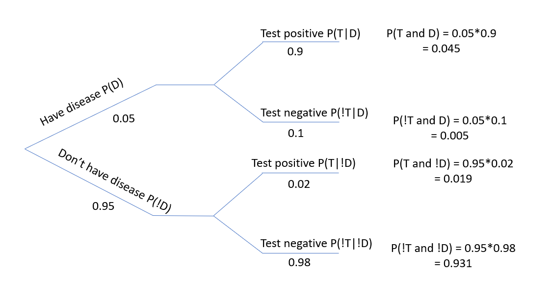
Figure 5.1: Tree diagram showing conditional probabilities.
Next, to find the joint probabilities, we generally work left to right, going along the various branches, where we multiply the individual probabilities along the path to that point. So on the top most branch \(P(T\ and\ D) = P(D)*P(T|D)\).
From here, once all the joint probabilities are known, you can employ our initial definition of conditional probability to find the value of interest.
Some people finding visualizing it in this manner makes it easier to understand and to work through what’s happening.
Note that if you were given the joint probabilities and either the marginal or conditional probabilities, you could then find the missing values.
5.4.1 Guided Practice
Bayes' rule can be used to assist with spam email filtering. In this problem you will compute the probability that an email message is spam, given that certain word appears in the message. Let:
- \(W\) be the event that a particular email has a given word, and
- \(S\) be the event that a particular email is spam.
We could then write an equation for \(P(S|W)\) assuming you knew the probability of a spam email containing the chosen word, such as "free", as well as the overall probability of receiving spam and the probability of all emails containing that specific word.
Now, assume the word is “free”. Assume the overall probability an email is spam 0.2, and the probability that an email contains the word free is 0.12. Also assume that the 40% of spam emails contain the word “free”.
What is the probability an email is spam given it contains the word "free"?
5.4.2 Drawing Probability Trees
It typically does not matter which variable is used as the marginal variable and which is used as the conditional variable, unless there is an obvious reason to choose one vs. the other. For example, in testing data, where we’re often given the false negative rates, it is easier to make the test result the conditional variable. Similarly, in the spam filtering problem we knew the probability of an email being spam given it contained the word free, so it made more sense to have the probability of containing the word free be the marginal variable.
Attempt to draw a probability tree for the following problem (the solution follows in the next section). Make sure to fill in the marginal, conditional and joint probabilities.
A company screens job applicants for illegal drug use at a certain stage of their hiring process. The specific test they use has a false positive (i.e. test returns positive when applicant is not using drugs) rate of 2% and a false negative (i.e. returns negative when applicant is using drugs) rate of 1%. Suppose that 8% of their applicants are actually using illegal drugs.
Let event \(A\) be the event whether the applicant is a drug user and event \(T\) be the even of whether the test comes back positive.
Create a tree showing \(P(A)\) and \(P(!A)\) as the marginal probabilities. I'd suggest you sketch this quickly by hand, but feel free to use a drawing program if that is easier for you.
5.4.3 Solution
Here is a possible probability tree for the previous problem, showing the marginal, conditional and joint probabilities:
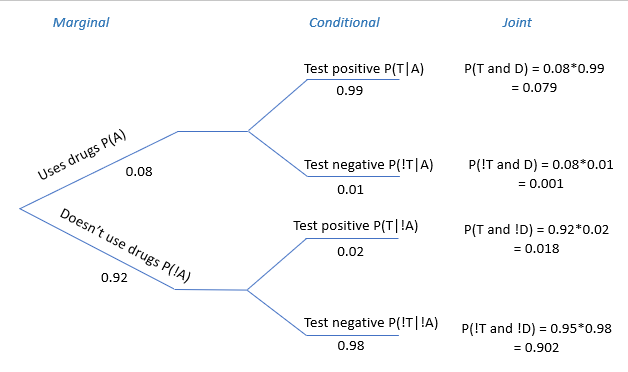
Figure 5.2: Spam Filtering probability tree diagram.
5.5 Review
| Name | Equation |
|---|---|
| Marginal and Joint Probabilities | \(P(A) = P(A\ and\ B) + P(A\ and\ !B)\) |
| Conditional Probability | \(P(A|B) = \frac{P(A\ and\ B)}{P(B)}\) |
| General Multiplication Rule | \(P(A\ and\ B) = P(A|B)*P(B)\) |
| Sum of Conditional Probabilities | \(P(A_1|B) + P(A_2|B) + ... P(A_n|B) = 1\) |
| Bayes Theorem | \(P(B|A) = \frac{P(A|B)P(B)}{P(A)} = \frac{P(A|B)P(B)}{P(A|B)P(B) + P(A|!B)*P(!B)}\) |
- and make sure to understand how these simplify under the assumption of independence.
5.5.1 Review of Learning Objectives
By the end of this chapter you should be able to
- Define conditional probability and give examples where it might be useful
- Explain and use the sum of conditional probabilities rule and the general multiplication rule
- Define Bayes’ rule and calculate conditional probabilities using Bayes’ rule
- Draw and use tree diagrams to represent conditional probabilities
5.6 Exercises
Note: These are not required and will occasionally be used during class as warm-up exercises or no-stakes quizzes.
Exercise 5.1 For two events, $A and $B, let \(P(A) = 0.3\) and \(P(B) = 0.7\)
- Can you compute \(P(A\ and\ B)\) if you only know \(P(A)\) and \(P(B)\)?
- If events \(A\) and \(B\) arise independently, what is \(P(A\ and\ B)\)?
- If events \(A\) and \(B\) arise independently, what is \(P(A\ or\ B)\)?
- If events \(A\) and \(B\) arise independently, what is \(P(A|B)\)?
Exercise 5.2 Suppose 80% of people like peanut butter, 89% like jelly, and 78% like both.
- Define your events using probability notation.
- Given that a randomly sampled person likes peanut butter, what’s the probability that he/she also likes jelly? Write this in probability notation and calculate the answer.
- Given that a randomly sampled person doesn’t likes peanut butter, what’s the probability that he/she also doesn’t like jelly? Write this in probability notation and calculate the answer.
- Does it seem liking peanut butter and liking jelly are independent of one another?
Exercise 5.3 Event \(A\) has three possible outcomes: \(A_1\), \(A_2\) and \(A_3\). If \(P(A_1|B) = 0.4\) and \(P(A_3|B) = 0.3\), and \(P(B) = 0.1\), what is \(P(A_2|B)\)?
Exercise 5.4 The following table shows counts of gun ownership by state in the PNW for 399 randomly sampled people. Note the proportions of people per state are roughly the relative to the state populations.
| num of people | WA | OR | ID | MT | |
|---|---|---|---|---|---|
| don’t own a gun | 149 | 84 | 21 | 14 | |
| own one or more gun | 58 | 31 | 27 | 15 |
- Convert this table to proportions.
- Does your table suggest independence between gun ownership and state? Pick at least two cells to evaluate.
- If a randomly sampled person owns a gun, what is the probability they are from ID or MT?
- If a randomly sampled person is from OR or WA, what is the probability that they don’t own a gun?
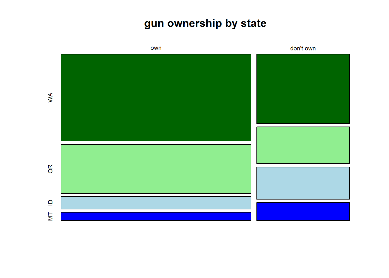
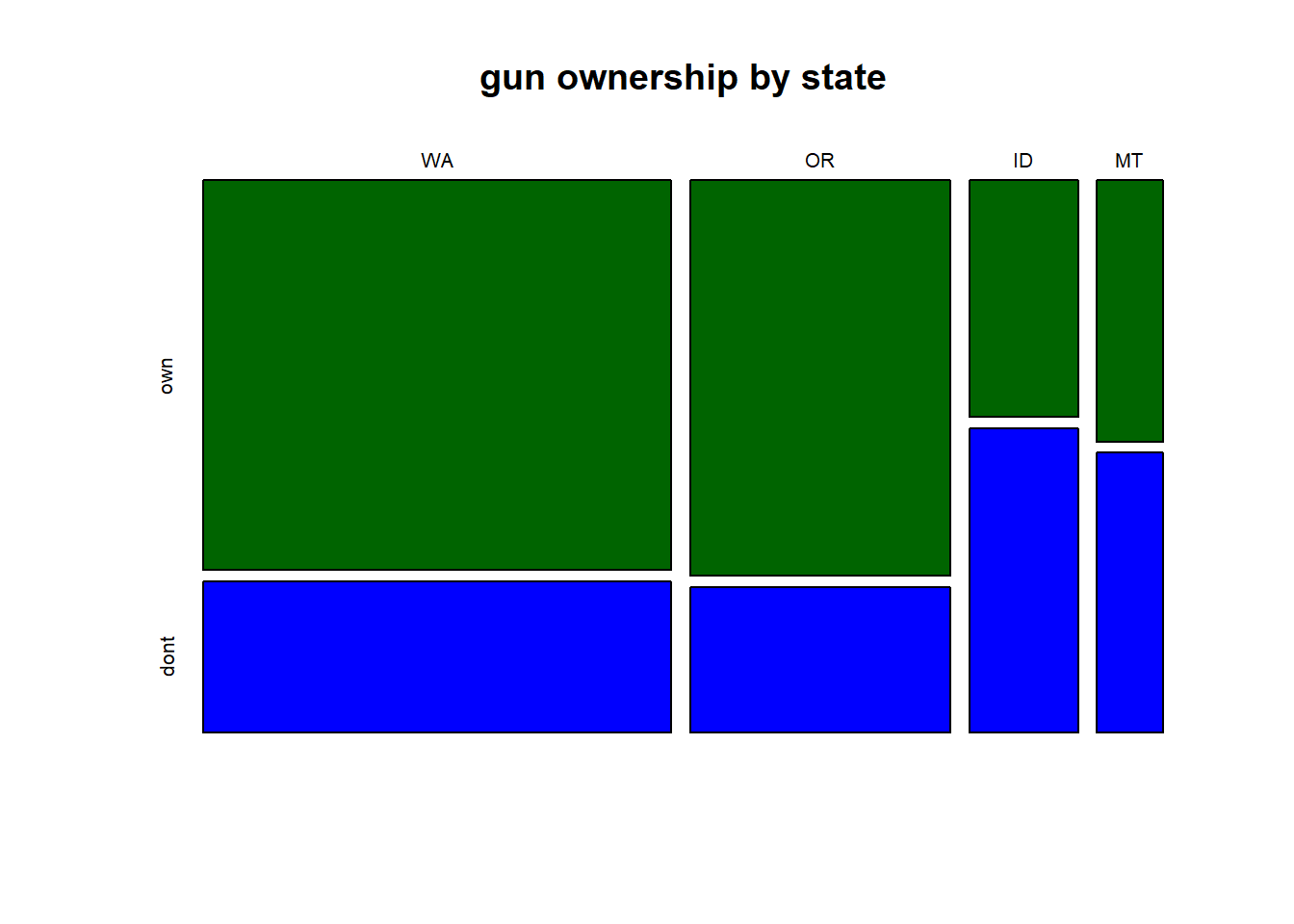
Exercise 5.5 The following two mosaic plots show the relationship between gun ownership and state, using the data from a previous exercise. Describe in a few sentences what each plots shows, including any interesting trends or patterns. Which plot is most useful to understanding the relationship between gun ownership and state, and why?
Exercise 5.6 After an introductory statistics course, 80% of students can successfully construct box plots. Of those who can construct box plots, 86% passed, while only 65% of those students who could not construct box plots passed.
(Hint: you may find it useful to create a 2x2 table to answer this problem.)
- Define your two events, and write the each of the probabilities listed above using probability notation.
- Given that a student passed, what is the probability that she is able to construct a box plot? Write this in probability notation and calculate the answer.
- Given that a student cannot construct a box plot, what is the probability that he passed? Write this in probability notation and calculate the answer.
Exercise 5.7 Edison Research gathered exit poll results from several sources for the Wisconsin recall election of Scott Walker in 2012. They found that 53% of respondents voted in favor of Scott Walker. Additionally, they estimated that of those who did vote in favor for Scott Walker, 37% had a college degree, while 44% of those who voted against Scott Walker had a college degree. Suppose we randomly sampled a person who participated in the exit poll and found that she had a college degree. What is the probability that she voted in favor of Scott Walker?
5.6.1 Bayes’ Rule
Exercise 5.8 Bayes rule can be used to assist with spam email filtering. In this problem you will compute the probability that an email message is spam, given that certain word appears in the message. Let \(W\) be the event that a particular email has a given word. Let \(S\) be the event that a particular email is spam.
Write the equation for \(P(S|W)\) assuming you knew the probability of a spam email containing the chosen word, as well as the overall probability of receiving spam and the probability of all emails containing that specific word.
Now, assume the word is “free”. Assume the overall probability an email is spam 0.2, and the probability that an email contains the word free is 0.12. Also assume that the 40% of spam emails contain the word “free”. What is the probability an email is spam given it contains the word “free”?
Exercise 5.9 Sore throat and congestion are symptoms of both the common cold as well as COVID-19. Let’s suppose that 95% of sick children in our region have the common cold and only 5% have COVID. We will assume no other illnesses in the area cause these symptoms.
Assume the probability of having both a sore throat and congestion if one has the common cold is 90%, whereas the probability of having both a sore throat and congestion if one has COVID is 30%.
If a child has a sore throat and congestion, what is the probability that they have the common cold?
Exercise 5.10 Suppose there is a certain disease, the probability of which an adult male in the general populations of having is \(P(D) = 0.05\). Assume the true positive rate is \(P(T|D) =0.98\) and the true negative rate is \(P(!T|!D) = 0.99\).
What is the probability an individual has the disease if their test came back positive? (i.e. calculate \(P(D|T)\))
Exercise 5.11 The parking lot at EPS is often full in the evenings. There are academic and recruiting events on 25% of evenings, sporting and theater events 30% of evenings, and no events on 45% of evenings. When there is an academic or recruiting event, the parking lot fills up about 25% of the time, and it fills up 70% of the evenings with sporting or theater events. On evenings with no events, it only fills up about 2% of the time. If someone visits the school and finds the parking lot full, what is the probability there is a sporting or theater event?
Exercise 5.12 Do the other two Bayes Rule examples from class that your group didn’t complete.
Exercise 5.13 In Canada, about 0.35% of women over 40 will develop breast cancer in any given year. A common screening test for breast cancer is the mammogram, but this test is not perfect. In about 11% of patients with breast cancer, this gives a false negative. Similarly, the test gives a false positive in 7% of patients who do not have breast cancer. If a test comes back positive, what is the probability that the patient actually has cancer?
Exercise 5.14 Joe is a randomly chosen member of a large population in which 3% are heroin users. Joe tests positive for heroin in a drug test that correctly identifies users 95% of the time (aka “sensitivity”) and correctly identifies nonusers 90% of the time (aka “specificity”). Determine the probability that Joe uses heroin (= H) given the positive test result (= E),
- What are the false positive and false negative test rates? Write these both as probability statements and calculate the values.
- What is the probability of a positive test result? Write this both as probability statements and calculate the value.
- What is the probability that Joe uses heroin given the positive test result? What do these results suggest to you?
- Bonus: Would taking the test again change the results? Why or why not?
(See: https://plato.stanford.edu/entries/bayes-theorem/supplement.html)