Chapter 18 Simple Linear Regression

18.1 Overview

In the previous two chapters we looked at evaluating whether there was a difference between multiple groups. Those groups might be thought of as potential predictor variables and then observed values were the response variables. For both chi-squared tests of homogeneity and for ANOVA tests, our null hypothesis was that the predictor variable (i.e. the group) had no influence on the average response. Said differently, the average response was the same for any of the predictors.

For both one way chi-squared tests and for ANOVA tests, the predictor variables are discrete or categorical, meaning they can only take certain values and are often grouped together. In this chapter, we will look at situation where we have continuous predictor variables.

This situation is commonly know as linear regression, which you probably encountered in Algebra 1 or 2. If we have a set of data that includes matching predictor and response values, both which are continuous, we often start with a scatter plot to see what type of relationship might exist. The question we’re often asking is: “Does the predictor variable tell me something about the response?” The simplest model (where we’ll start) is to assume (and test) a linear relationship.

At first glance, this may not seem like statistics. The equation of a line is \(y=mx+b\), where \(m\) and \(b\) are the slope and intercept parameters, respectively. However, rarely does all of our data fall right along the line. So, we will use statistics both (i) to find the values of \(m\) and \(b\) that lead the “best fitting line” (minimizes sum of square error) AND (ii) to test if the fitted value of \(m\) is significantly different than 0. If the slope is 0, it means that the predictor has no influence on the response, matching are null for both chi-squared testing and ANOVA.

18.2 A Quick Run through of Regression

In this section, we will give a quick run through of the major steps in performing linear regression, including:

• using scatter plots to visualize the relationship (and then adding our best fitted model/line),
• calculating correlation to quantify the linear relationship,
• creating a “linear model” in R using the lm() function,
  
• defining and plotting the residuals to assess model fit,
• interpreting the results of the summary() output,
• testing if \(\hat \beta_1\) (our estimate of the slope) is significantly different than 0,
• extracting the \(R^2\) value to understand effectiveness of the model, and
  
• using the model to predict new observations

18.2.1 Loading the data

For this introduction, we will use data collected by Mr. Derek Whiteside of the UK Building Research Station, who recorded the weekly gas consumption (1000s cubic ft) and average external temperature (degrees C) at his own house in south-east England in the 1960s. This data is available in the MASS library.

library(MASS)  ## we need to call this function to make the data available.

18.2.2 Scatter Plots and Correlatoin

Let’s start with a scatter plot, showing temperature on the x-axis and heating gas consumption on the y-axis. It seems reasonable to assume that as the outside temperature increases, the heating gas consumption might decrease.

plot(whiteside$Temp, whiteside$Gas, xlab="outside temp (C)", ylab="heating gas usage")

What do you notice? What type of relationship do you see and how would you describe it? Questions we will ask when evaluating scatter plots include:

• Does the relationship between x and y appear positive or negative (think about the slope)? Or does “no relationship” between the variables appear to exist (would the “best” slope likely be zero)?
  
• Is any observed relationship strong or weak? Here, think about if the points would fall right along a line or if they form a wider cloud around it.
  
• Does the relationship appear linear? Or is it exponential in shape or possibly some type of other curve?
  
• Does it appear that the variance (spread of the response data) is roughly the same as x increases?

Taking a step back, how did we decide which value to put on the \(x\) axis and which to put on the \(y\) axis? Generally here, and when possible, we’ll put the predictor variable on the x-axis and the response variable on the y-axis. In this case, its the outside temperature that influences the amount of heating gas used (not the other way around), so being the predictor variable, the temperature goes on the x-axis.

18.2.3 Correlation

We introduced the idea of correlation back in Chapter 3. As a reminder, correlation is a measure of the strength of the linear relationship between two variables. (And, similar to what we saw with boxplots, correlation can be useful to tell us some things but it isn’t perfect. In fact, you can have a high correlation even if the data do not have a linear relationship.)

The following calculates the correlation between outside temperature and heating gas usage:

cor(whiteside$Temp, whiteside$Gas)

## [1] -0.6832545

Generally a value of \(r=-0.683\) (and we typically use the variable \(r\) for correlation) suggests a moderately strong negative relationship. However, it is important to remember that this does NOT necessarily imply a “linear” relationship as we’ll see shortly. Nor does it imply causality.

18.2.4 Our Linear Model

Next, if we wanted to evaluate if there’s a “linear” relationship between temperature \(x\) and heating gas usage \(y\), we need to think about what our “model” is, namely:

\[y = \beta_0 + \beta_1 x + \epsilon\]

Where

• \(x,y\) are our data and in particular \(x\) is our “predictor” variable and \(y\) is our “response” variable
  
• \(\beta_0\) (intercept) and \(\beta_1\) (slope) are the model parameters (think \(b\) and \(m\) but in “statistics speak”)
• \(\epsilon\) is a measure of uncertainty, which is typically assumed to be Normally distributed

In this chapter we’ll learn how to estimate and interpret the coefficients: \(\beta_0\), \(\beta_1\) and \(\epsilon\).

Overall, goals of “simple linear regression” analysis include:

1. calculating the best values of \(\beta_0\) and \(\beta_1\), and
   
2. determining if a linear model is appropriate and how good of a model it is Here the term “simple” refers to that we only have a single predictor variable, not that the process is simple!

18.2.5 Fitting and Plotting Our Linear Model in R

To start, I’ll show you how to fit a linear model, then below in subsequent sections we’ll delve into the R commands and output in much more detail.

We’ll use a new R command here, lm(), which stands for “linear model” and acts somewhat similar to aov(). Note the use of the ~ character again, where here we’re modeling gas usage “as a function of” temperature.

whiteside.lm <- lm(Gas~Temp, data=whiteside)  ## create the linear model object

Since the results are stored in whiteside.lm, R doesn’t give us any output. Also note that the .lm extension is not required, it simply helps remind me that the variable is a linear model.

Next, let’s add the fitted line our scatter plot (which is really easy!):

plot(whiteside$Temp, whiteside$Gas, xlab="outside temp (C)", ylab="heating gas usage")  ## same as before
abline(whiteside.lm, col="red")  ## just use your fitted model object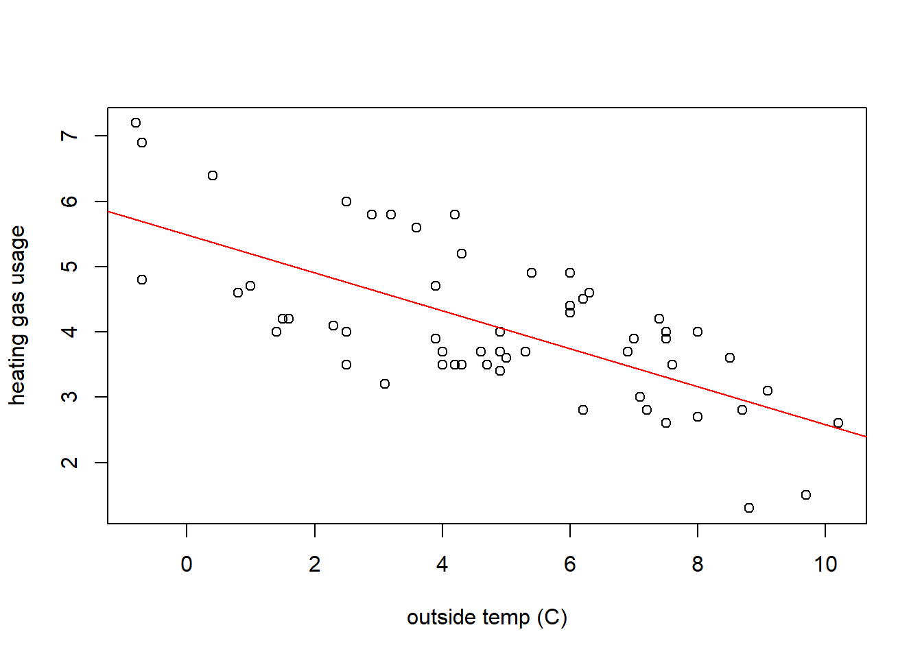

You may notice we’re using the abline() function in a slightly different manner here, and R is smart enough to figure out what we mean. Easy, right?

Based on this plot and fitted line, does it seem like our model is a “good fit”? How would you tell?

18.2.6 Residuals: Assessing Model Fit

From above, our model was: \(y = \beta_0 + \beta_1 x + \epsilon\). We can alternatively write this as “Data = Fitted + Residual”. Mathematically we might write this for each data point \(i\) as \[y_i = \hat y_i + \epsilon_i\]

where \(y_i\) is each observed data point, \(\hat y_i\) is the fitted value based on our model (on the line), and \(\epsilon_i\) is the error between our fitted and observed results.

We can rearrange this last equation as \(\epsilon_i = y_i - \hat y_i\) and the set of \(\epsilon_i\) are known as the residuals. Next, let’s plot just the residuals as a function of our \(x\) variable:

plot(whiteside$Temp, whiteside.lm$residuals, ylab="residuals")
abline(h=0, col="red", lty=2)

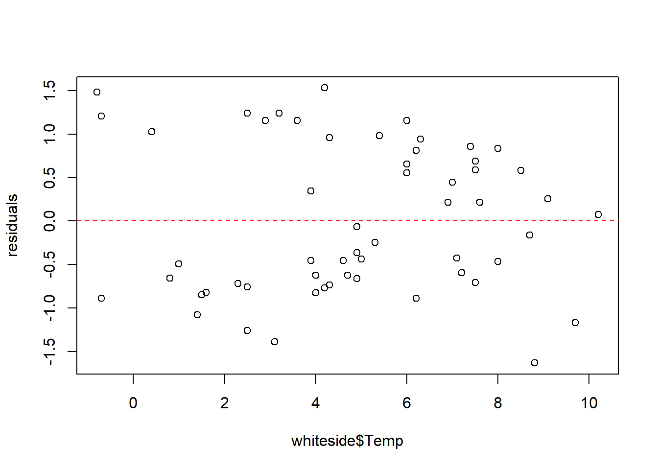
Our model assumes these to be randomly distributed and centered around 0 (which is why I’ve added a horizontal line at 0). What do you observe?

• Do the residuals show any trend as x increases?
  
• Our model assumes the residuals \(∼N(0,\epsilon)\). This will be particularly important for prediction. Is this what we observe?

Another way to look at the data (specifically to evalute the second bullet point) is using a histogram:

hist(whiteside.lm$residuals)

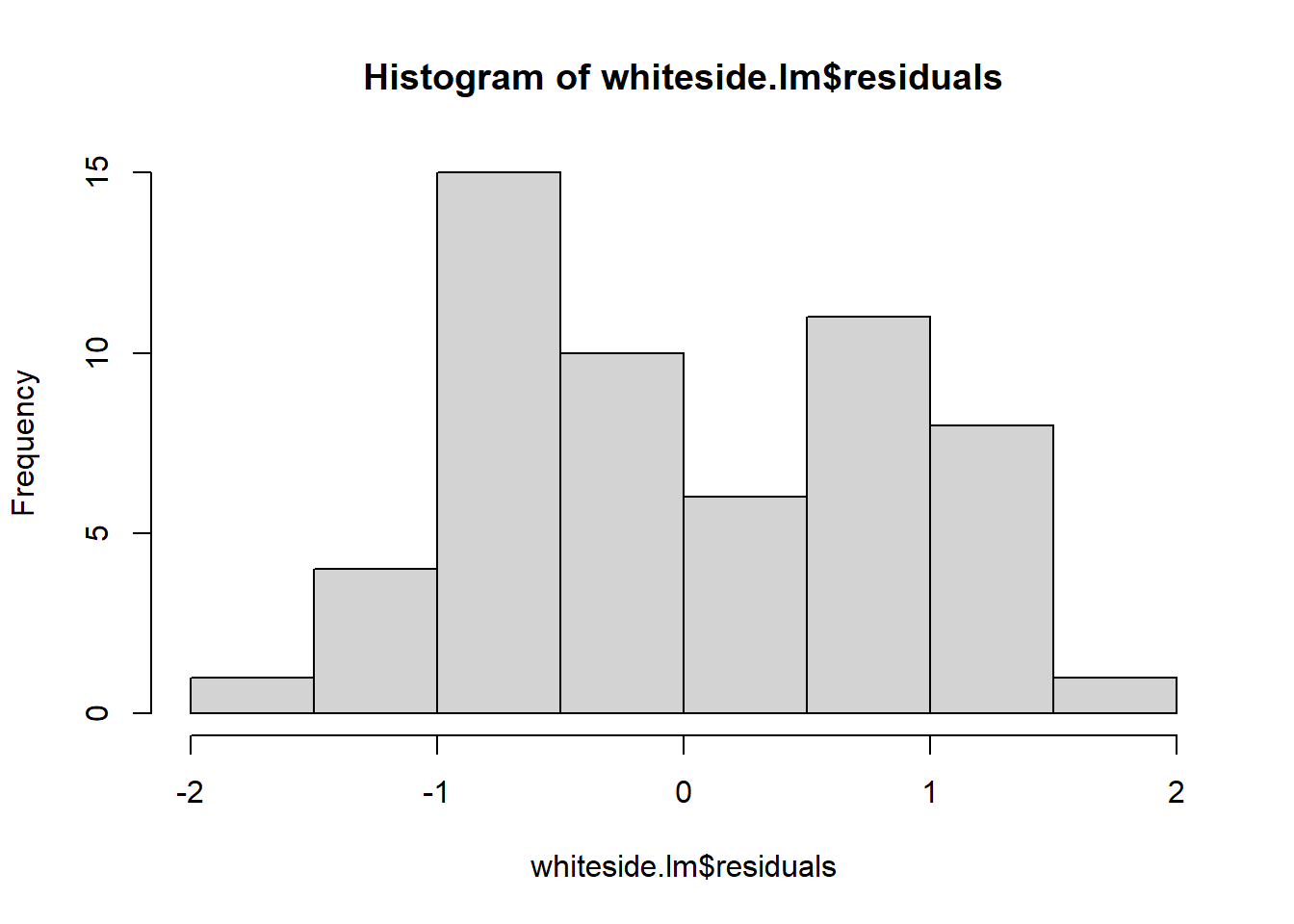
Remember that small sample sizes from Normal distributions don’t always appear exactly normal. Overall this fit looks “OK”, not perfect. We will dive deeper into this data in Chapter 19 to see why.

More generally, we’ll use residual plots as one approach to assess how good of a fit a linear model is.

18.2.7 The summary() Output

Now that we have decided a linear model might be a good fit, let’s look in more detail at our fitted model, using the summary() command:

summary(whiteside.lm)                         

## 
## Call:
## lm(formula = Gas ~ Temp, data = whiteside)
## 
## Residuals:
##     Min      1Q  Median      3Q     Max 
## -1.6324 -0.7119 -0.2047  0.8187  1.5327 
## 
## Coefficients:
##             Estimate Std. Error t value Pr(>|t|)    
## (Intercept)   5.4862     0.2357  23.275  < 2e-16 ***
## Temp         -0.2902     0.0422  -6.876 6.55e-09 ***
## ---
## Signif. codes:  0 '***' 0.001 '**' 0.01 '*' 0.05 '.' 0.1 ' ' 1
## 
## Residual standard error: 0.8606 on 54 degrees of freedom
## Multiple R-squared:  0.4668, Adjusted R-squared:  0.457 
## F-statistic: 47.28 on 1 and 54 DF,  p-value: 6.545e-09

As we saw with ANOVA, there’s a lot going on here! What’s most important? Under the Coefficients: table look at the Estimate and Pr(>|t|) columns.

One of our main questions will be to test \(H_0: \beta_1 = 0\). Why? Because \(\beta_1\) is the slope, and if the slope is not significantly different than 0, then there is NO relationship between the variables.

The Estimate column contains the estimates of \(\beta_0 = 5.48\) (the intercept) and \(\beta_1 = -0.290\) (the slope). Make sure you are clear on how to interpret these values! In this case, the slope means that for each degree increase in outside temperature, the heating oil usage goes down by \(-0.29\) thousand cu ft. Similarly, the intercept means that if the outside temperature were 0, the expected heating oil usage would be \(5.48\) thousand cu ft.

The Pr(>|t|) column tells us if these are each significantly different than 0. What’s shown are p-values testing each specific null hypothesis (\(\beta_i = 0\)). Since both p-values are lower than \(\alpha=0.05\), we would conclude that both the slope and intercept are “significant”, meaning non-zero. As we’ll see later on, in each case R is performing a one sample t-test.

One other statistic we’ll look at here is the \(R^2\) value. This tells us the percent of variation in \(y\) that is explained by our model. In this case, 46.7% of the variation in heating oil use is explained by temperature, so 53.3% is left unexplained. Better models will explain higher percentages, up to 100%.

18.2.8 Prediction

Lastly, if we decide that we are happy with the model fit, what do we do with it?

We might want to use this model to predict the response for a given predictor value, such as the gas usage at a temperature of 1 (degree C). How would we do that? Given our model parameters, we can just calculate this “by hand” (where I’m accessing the coefficients vector) as:

## Extract the coefficients
beta0 <- unname(whiteside.lm$coefficients[1])
beta1 <- unname(whiteside.lm$coefficients[2])
## What does our linear models say if temp = 1?
beta0 + beta1*1

## [1] 5.195985

The unname() function is unnecessary, and simply removes the names from the elements of the vector.

Here we’re extracting the values of \(\beta_0\) and \(\beta_1\) from our model, and using those to calculate the value of y as: \(y= \beta_0 + \beta_1 x\) for a value of \(x=1\).

Unfortunately, we’re pretty sure this prediction will be wrong. Why? Because as our model, data and residuals show, (almost) none of the observed points fell right on the regression line.

So, in addition to a point estimate, we should also give an estimate of the uncertainty in our prediction. We’ll do this with the predict.lm() function in R:

newx <- data.frame(Temp=c(1))   # need to create this as a data.frame()
predict.lm(whiteside.lm, newdata= newx, interval="prediction")

##        fit      lwr      upr
## 1 5.195985 3.424623 6.967348

This creates a 95% confidence interval on how much heating oil would be used (the response) if the predictor was 1 degree C, namely between 3,425 and 6,967 ft\(^3\).

We’ll talk later about differences between ‘prediction’ intervals and ‘confidence’ intervals. In short, are you interested in predicting the range where the average result would lie? Or the range where an individual value might lie? You should think about why those might be different.

18.2.9 Summary and Review

The goal of this introductory section was to provide a quick overview of the linear regression process including:

• using scatter plots to visualize the relationship (and then adding our best fitted model/line),
• calculating correlation to quantify the linear relationship,
• creating a “linear model” in R using the lm() function,
  
• defining and plotting the residuals to assess model fit,
• interpreting the results of the summary() output,
• testing if \(\hat \beta_1\) (our estimate of the slope) is significantly different than 0,
• extracting the \(R^2\) value to understand effectiveness of the model, and
  
• using the model to predict new observations

These are the topics we will delve further into throughout the remainder of this chapter.

18.3 Scatter Plots and Correlation

In this section we will reintroduce the methods of creating scatter plots and calculating and interpreting the correlation between variables, along with discussing the difference between correlation and causation. Some of this will be review from section 3.9, and students should refresh their knowledge as necessary.

Creating scatter plots and calculating the correlation between variables is often the first few steps in a regression analysis, as they can help visualize and evaluate whether a linear relationship might exist between our variables.

By the end of this section you should be able to:

• Create “well-formatted” scatter plots showing the relationship between two continuous variables and interpret the observed relationship
  
• Defend your choice of predictor vs. response variables (or dependent vs independent variables) when creating scatter plots
  
• Describe the relationship between two variables
  
• Explain (generally) what correlation calculates
  
• Calculate the correlation of two variables in R and interpret the results. (Hint: be aware of use="p" if NA exist.)
  
• Discuss if and when a strong correlation implies a good linear fit
  
• Describe the tenuous relationship between correlation vs. causation

18.3.1 Creating Scatterplots

A scatter plot is a plot of two variables on the same plot, and in R we simply use the plot() function to create it.

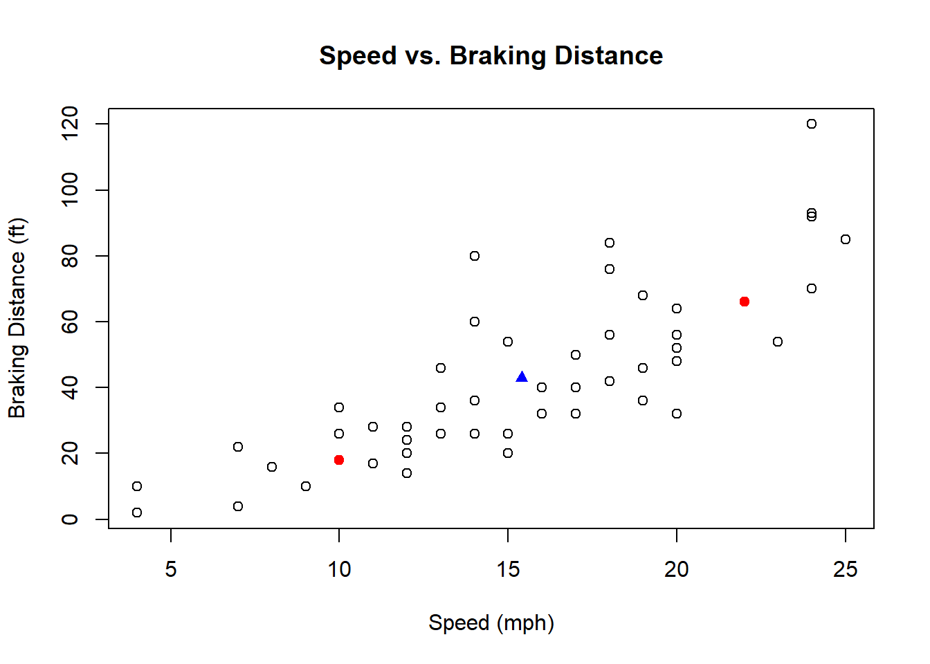
Here we’ll look at the cars dataset, which contains information about speed and braking distance for a variety of cars. More information the data itself can be found by typing ?cars at the console. The columns names $speed and $dist are found as:

names(cars)

## [1] "speed" "dist"

A scatter plot of this using speed as our predictor variable (x-axis) and distance as our response variable (y-axis) is created using:

plot(cars$speed, cars$dist, xlab="Speed (mph)", ylab="Braking Distance (ft)", main="Speed vs. Braking Distance", col="blue", pch=19, xlim=c(0,30))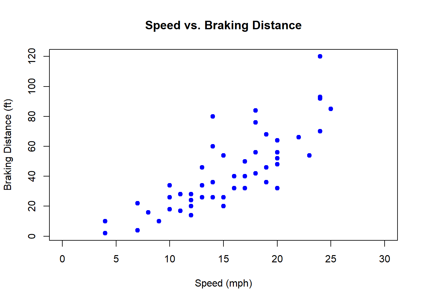

Here we observe that braking distance generally increases as speed increases, although there is some uncertainty in the results.

More generally, how do we choose which variable to put on the x-axis versus on the y-axis?

The terms predictor and response variables were introduced above. The idea is that for the given relationship, the predictor helps determine the response. It is customary to put the predictor on the x-axis and the response on the y-axis. In this case it seems clear that speed is the predictor of braking distance.

Note that these might also be referred to as independent (x) vs dependent (y) variables.

18.3.2 Customizing Scatter Plots

R has a lot of capabilities to customize scatter plots, including parameters to the plot() function as well as additional functions that can be called after the plot has already been created.

Some useful parameters to the plot() function:

• change the color using col
• change the plotting character using pch
• adjust the x- and y-axis ranges using xlim and ylim

Additional functions to customize an existing plot:

• add custom text using the text() function
• add a legend using the legend() function
• add additional points using the points() function

We’ll use the latter set of these more when we’re looking at multiple linear regression.

For additional details about how to further customize plots, look at ?plot and ?par

18.3.3 Describing Scatter Plots

Let’s dive further into the above plot of speed vs. braking distance. How would we describe this relationship? Interpreting scatter plots is a critical skill that we need to learn. Some guiding questions you should attempt to answer while looking at this graph (and similar) include:

• Does the relationship between x and y appear positive or negative (think about the slope)? Or does “no relationship” between the variables appear to exist (in which case the “best slope” would be zero)?
• Would you describe any observed relationship as strong or weak? Here, think about if the points would fall right along a line or if they form a wider cloud around it.
• Does the relationship appear linear across the range of \(x\) values? Or is it exponential in shape or possibly some type of other curve?
• Does it appear that the variance (spread of the response data in the \(y\) direction) is roughly the same as \(x\) increases?

18.3.4 Guided Practice

For each of the following plots, describe the relationship between \(x\) and \(y\) using the above four (4) questions as a guide:

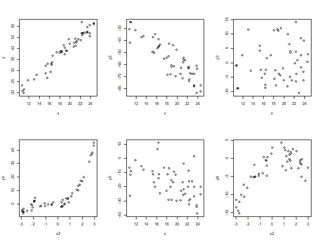
Figure 18.1: Scatterplots showing different relationships and correlations.

18.3.5 The Correlation of Different Scatter Plots

Above we discussed some qualitative approaches to evaluating scatter plots. Here, we’ll remind ourselves of one of the main quantitative measures we use of determining the strength of a linear relationship, namely the correlation.

Correlation was introduced in Chapter 3. As a reminder, it is a measure of the strength of a linear relationship between two variables, and ranges between 1 and -1.

Repeating the graphic from Chapter 3:

Figure 18.2: The relationship between scatterplots and correlation value from mathisfun.com

This shows how the calculated correlation value relates to both whether a relationship is positive or negative and it’s strength.

18.3.6 Guided Practice

Match each of the scatter plots from the previous Guided Practice with their correlation value.

1. -0.878
2. -0.478
3. -0.194
4. 0.128
5. 0.706
6. 0.975

One important take-away from this is in how we should interpret calculated correlation values. They can be informative, but only up to a point, particularly if our goal is to evaluate whether a linear relationship exists between \(x\) and \(y\).

18.3.7 Optional: How is Correlation Calculated?

The equation for variance should be very familiar by now:

\[\sigma^2 = \frac{1}{n} \sum_{i=1}^n(x_i-\bar x)^2\]

If we have \(n\) data points, then variance is a measure of how far every point \(x_i\) is away from the mean \(\bar x\), and that value is squared, summed, and then scaled by the number of data points.

Written in a similar form, the equation for correlation is:

\[cor(x,y) = \frac{1}{n-1} \sum_{i=1}^n\frac{(x_i-\bar x)}{\sigma_x}\frac{(y_i-\bar y)}{\sigma_y}\]

This is certainly a similarity to variance, and the important differences are:

1. the \(y\) values are now included, and
   
2. we scale each difference (e.g. \((x_i-\bar x)\)) by its standard deviation (\(\sigma_x\)).

The advantage of scaling is two-fold. First, because the standard deviation has the same units as the data, the covariance becomes unitless. Second, because of this scaling, the resulting values will range between -1 and 1. (For those of you who want to dive deeper here, look into the equation for covariance.)

To understand what the correlation equation does, I find it useful to consider a few different cases, an in particular look at the product \((x_i-\bar x)(y_i-\bar x)\):

• What if \(x\) and \(y\) have a strong positive linear relationship? In that case, as \(x\) gets large compared to \(\bar x\), \(y\) also gets large compared with \(\bar y\). So, in the covariance equation, both values are positive, multiplied together. A similar positive result happens if both \(x\) and \(y\) get small compared to their means. The sum of all of these will reinforce to a strong positive value (close to +1)
• Alternatively, if \(x\) and \(y\) have a strong negative linear relationship, the product will be negative, and the sum of all of these will reinforce to a strong negative value (close to -1)
• Finally, if there is no relationship between \(x\) and \(y\), then the products will vary. Some will be positive and some will be negative. Summing these will lead to a result that averages out close to 0.

As a specific example, the blue triangle below shows the mean \(\bar x, \bar y\) as well as two red points. Work through the above ideas for those two red points to see their contribution to the correlation.

18.3.8 Calculating Correlation

We can calculate correlation between the speed and braking distance in R as:

cor(cars$speed, cars$dist, use="p")

## [1] 0.8068949

(NOTE: Sometimes when we use real data, there are missing observations. R typically represents this as “NA”. The use="p" parameter tells R to only include those data points for which both observations exist. You may need this for the homework. )

How do we interpret the value of \(0.807\)? As mentioned above, because we’re scaling by the two standard deviations, our \(r\) value will always be between -1 and 1. Values closer to 1 suggest stronger correlation between the variables.

So, the computed correlation value of \(r=0.807\) suggests a pretty strong linear relationship between speed and braking distance.

18.3.9 Does High Correlation Imply a Linear Fit?

If we calculate a high correlation (either close to 1 or -1), does that mean a linear model is appropriate?

Not necessarily. Because of how it’s calculated, as long as there’s a positive (or negative) relationship between the variables, the correlation may be high. This was illustrated in the guided practice above.

As another example, inspect the following plot:

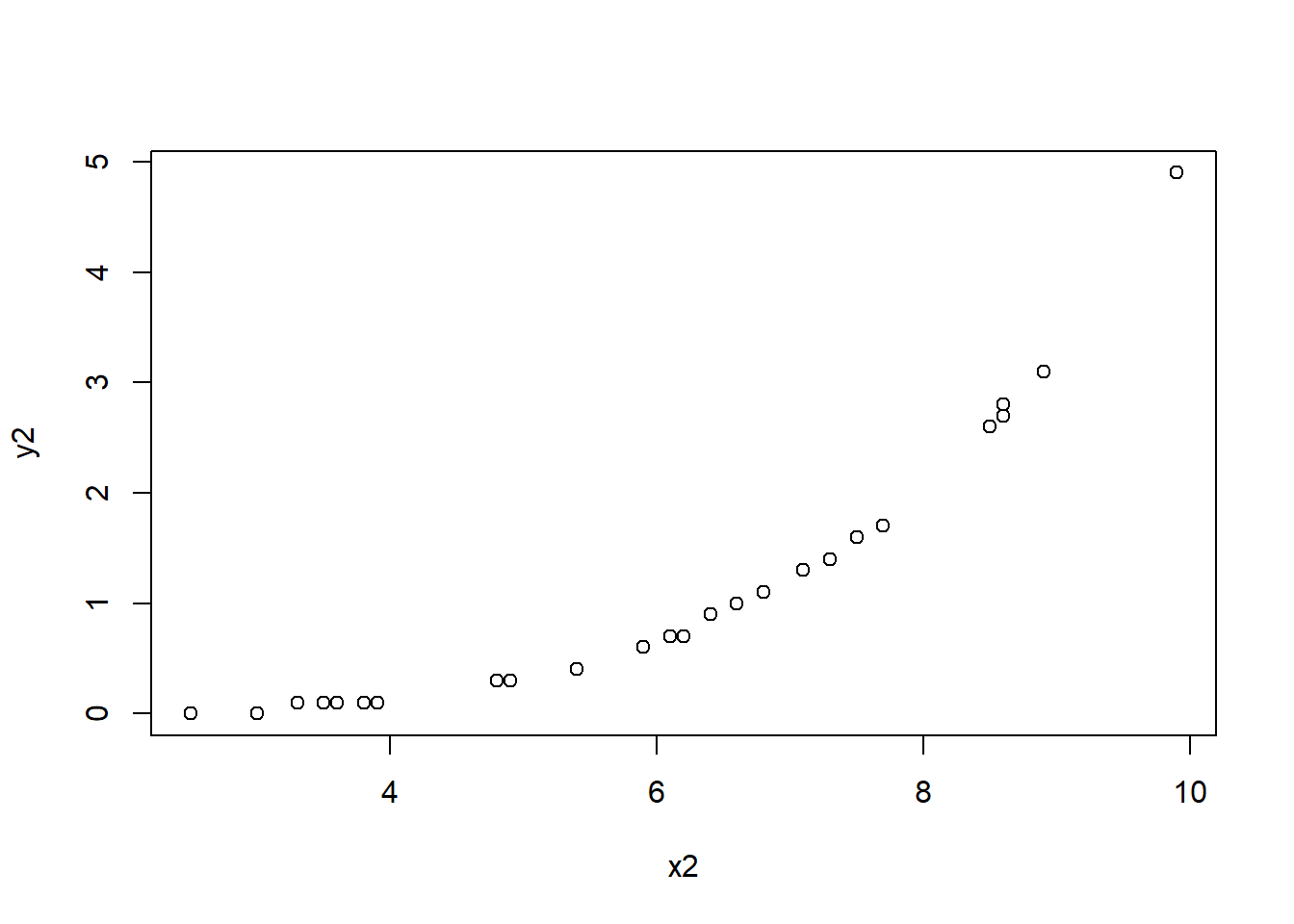
Calculating the correlation between these values we see it shows strong correlation exists:

cor(x2, y2)

## [1] 0.9073204

However, the plot is clearly NOT linear. So, importantly, finding a high correlation is necessary but not sufficient toward evaluating if a strong linear relationship exists. At a minimum you should confirm the scatter plot shows a roughly linear relationship, and we’ll see additional methods below to help evaluate this.

18.3.10 Correlation vs. Causation

What is the relationship between a high correlation value and whether causation exist? In other words, does a high correlation necessarily imply that variable \(x\) causes variable \(y\)? In a word, NO.

Watch this video from Khan Academy (10:44): https://www.khanacademy.org/math/statistics-probability/designing-studies/sampling-and-surveys/v/correlation-and-causality

What does Sal suggest as a possible underlying variable that might cause both eating breakfast and not becoming obese?

The takeaway is that high correlation does NOT imply that one variable causes the other. And, without fully understanding the “system” behind our variables of interest, it can often be difficult to figure out whether variable \(A\) might cause variable \(B\) or the other way around, or if some other, unmeasured variable \(C\) might be causing both.

Some important points:

• Just because we can plot two variables together does NOT mean a causal relationship exists.
• Just because a high (i.e. close to 1 or -1) correlation exists between two variables, does NOT mean a causal relationship exists.

Again, there may be some unknown covariate that impacts both, or maybe not. As a statistician, you need to pull back from the math and use reason and logic to evaluate whether a causal link between the two variables makes sense.

Imagine the following scenarios, where a high correlation is presumed to exist in both cases:

1. If I study hard, I’ll probably get good grades. (Here studying hard causes you to learn the material, which causes you to get good grades - the causal link makes sense.)
   
2. If I do lot’s of extracurricular activities, I’ll probably get good grades. (Here, maybe, but the causal link is certainly weaker. Students who participate in lots of extracurricular activities might have less time to study which could negatively impact their grades. Or, maybe the people who are driven to do lots of extracurricular activities are also driven to study hard? The causal link is weaker here, and probably any correlation is in fact driven by some third variable, e.g. desire to get into a good college.)

Also, be wary of cases where time is the predictor. For example, does time cause more CO\(_2\) to be emitted into the atmosphere? Not really, but a plot would show high correlation between these. It’s more likely that since economic growth also generally increases over time, and given CO\(_2\) emissions and economic growth are related, we can thus reason through why CO\(_2\) emissions are correlated with time.

Lastly, as another example, check out this Harvard Business Review article discussing examples of spurious correlation: https://hbr.org/2015/06/beware-spurious-correlations.

18.3.11 Summary and Review

By the end of this section you should be able to:

• Create “well-formatted” scatter plots showing the relationship between two continuous variables and interpret the observed relationship
  
• Defend your choice of predictor vs. response variables (or dependent vs independent variables) when creating scatter plots
  
• Describe the relationship between two variables
  
• Explain (generally) what correlation calculates
  
• Calculate the correlation of two variables in R and interpret the results. (Hint: be aware of use="p" if NA exist.)
  
• Discuss if and when a strong correlation implies a good linear fit
  
• Describe the tenuous relationship between correlation vs. causation

18.4 Our Linear Model

Now we are ready to dive into the details of what a “linear model” means and how to fit and evaluate one in R. By the end of this section you should be able to:

• Fit a linear model using the lm() function in R and extract the slope and intercepts coefficients of the best fitting line.
• Understand what is meant by “best fitting line” and “least squares regression”, namely that these lines minimize the sum of squared residuals, \(\sum \epsilon_i^2\)
• Interpret the slope and intercept coefficients in terms of the original data
• Overlay the fitted line onto a scatter plot of the data
• Define the terms “observed data”, “fitted data” and “residuals”, and both describe how they relate to our “model” as well as how they relate to one another
• Calculate or extract the residuals and plot them to evaluate if the assumptions of no bias or trend, random distribution and constant variance seems reasonable

18.4.1 What is a “model”?

What is meant by our “model”? The model is our representation of the relationship between the predictor and response variables. As was introduced above, we will use a linear model of the form:

\[y=\beta_0 + \beta_1 x + \epsilon\]

Where:

• \(x,y\) are our given data - here \(x\) is a vector our chosen predictor variable and \(y\) is a vector our response variable
• \(\beta_0\) and \(\beta_1\) are the model coefficients that represent the intercept and slope, respectively
• \(\epsilon\) is a vector that measures the uncertainty of each fitted value, which as discussed below will assumed to be Normally distributed

An alternative form of this model is::

\[y_i=\beta_0 + \beta_1 x_i + \epsilon_i\]

where here the index \(i\) refers to each specific data point.

Statisticians use \(\beta_0\) and \(\beta_1\) instead of \(b\) and \(m\), but they are equivalent.

A word on the uncertainty. We don’t expect (or require) that the relationship between \(x\) and \(y\) is perfectly linear. All the points don’t need to fall right along the line. The \(\epsilon\) term accounts for that.

An alternative, but equivalent, form of our model is to represent our observed data as: Data (\(y\)) = Fitted (\(\beta_0 + \beta_1 x\)) + Residual (\(\epsilon\)). This form more clearly separates the line (fitted) from the uncertainty (residual).

In this section I will show how these different forms are equivalent, and where each is useful.

Overall, our goals of linear regression are typically to:

• figure out the best estimates of \(\beta_0\), \(\beta_1\) and \(\epsilon\),
• determine if a linear model is a good fit, and if so,
• use this model for prediction of new values

We will walk through each of these steps in the remainder of this chapter.

18.4.2 Example Data

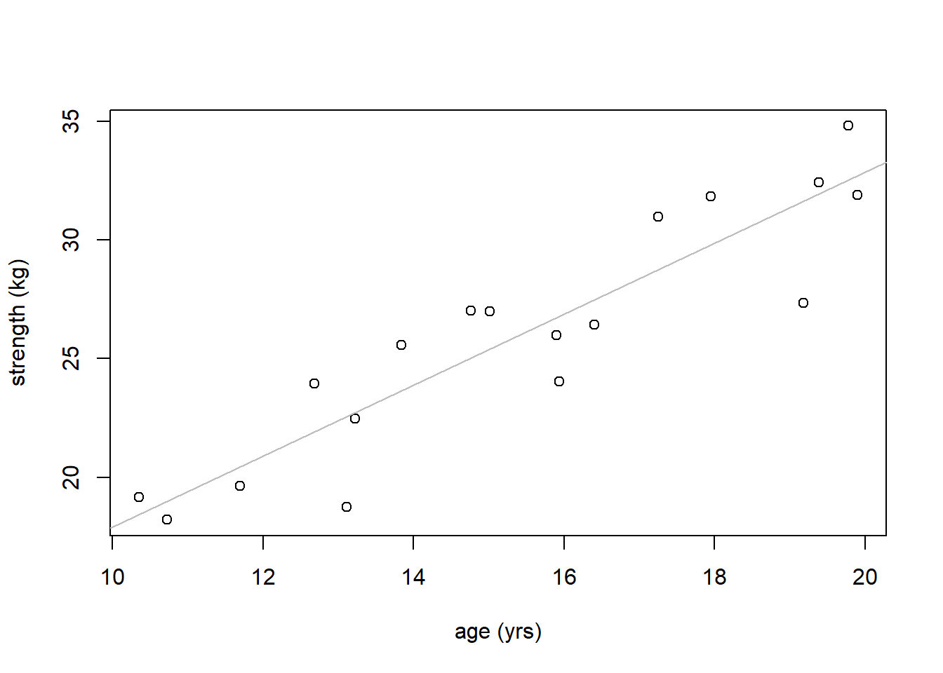
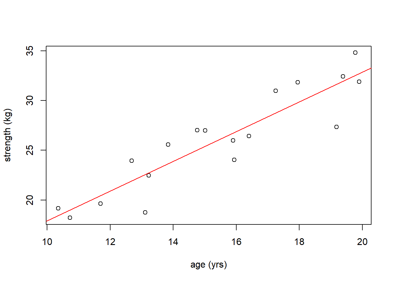
Suppose we have the following data which measured strength a function of age for a population of girls. Since age is a possible predictor of strength, we’ll set age as the \(x\) variable and strength as the \(y\) variable.

age <- c(19.39, 10.72, 10.35, 19.78, 15.94, 17.95, 15.90, 19.90, 15.01, 13.22, 11.69, 16.40, 13.84, 14.76, 12.68, 13.11, 17.25, 19.18)
strength <- c(32.42, 18.21, 19.16, 34.80, 24.04, 31.83, 25.99, 31.89, 27.00, 22.47, 19.63, 26.44, 25.56, 27.03, 23.93, 18.74, 30.98, 27.35)
plot(age, strength, xlab="age (yrs)", ylab="strength (kg)")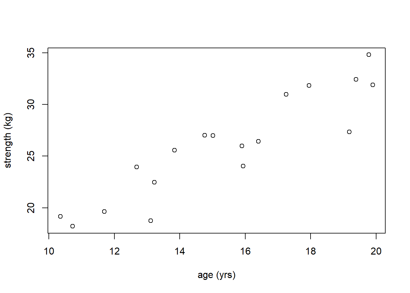

First, before we get started, how would you describe this relationship? Answers should include:

• mostly linear at least across the ages measured,
• a positive (increasing) relationship,
• fairly strong linear relationship since the points all fall close to the probable regression line.
• constant variance in \(y\) across the different values of \(x\) (look at this as vertical slices)

18.4.3 Determining the Model Coefficients

Given that it seems a linear relationship might be reasonable here, let’s proceed to determine the model.

In R, similar to our ANOVA call, we use lm() with the ~ character to represent “as a function of”. We want to fit a model with \(y\) as a function of \(x\).

## Create our linear model, I'll typically make this its own variable
str_age.lm <- lm(strength~age)      

Note that we can call our model whatever we like - I tend to include the *.lm so that I know it’s a linear model object.

Once we have our model, we can extract the values of the coefficients as:

## Extract the coefficients
str_age.lm$coefficients    

## (Intercept)         age 
##     2.93450     1.49655

What do these values represent? These are \(\beta_0\) and \(\beta_1\).

If I ask you to interpret the parameters, here’s what I’m looking for:

• the slope value (age) means that for each unit increase in age (yr) the average strength increases by 1.497 units (kg).
  
• the intercept value (Intercept) means that if age were 0, the strength would be 2.93 units. Note that sometimes the interpretation of intercept is a bit nonsensical. In such cases, as we have here, you can think of it as helping locate the line. Note in particular we don’t have any data near \(x=0\) so making inference about strength corresponding to that age would be inappropriate.

So, at this point, we have our fitted line, which we might write (within rounding) as \(y = 1.49 x + 2.93\). This does not (yet) consider the uncertainty or error that exists.

We can plot the fitted line on our scatter plot using the abline() function. R is smart enough to figure out what we intend:

plot(age, strength, xlab="age (yrs)", ylab="strength (kg)")
abline(str_age.lm, col="gray")

Does the fitted line seem appropriate? We’ll discuss this shortly.

NOTE: if your fitted line doesn’t at least somewhat go through the center of your points, you’ve likely done something wrong. A common mistake that causes this is when the model is fit backwards (e.g. age~strength).

For general data \(x\) and \(y\), note the order of the parameters in the plot() and lm() functions as:

# Not run
plot(x, y)                  # here x-axis data goes first then y-axis data
example.lm <- lm(y ~ x)     # here we model y "as a function of" x

18.4.4 Guided Practice

Find the slope and intercept parameter for relationship between speed and braking distance in the cars data. Interpret the values in context.

18.4.5 A Technical Note about lm()

The lm() call returns an R object which is a list. You can access lists similar to how you use dataframes, including the names() function and the $. But note, the results here are not columns in a matrix, but instead elements of the list, but you access them the same way.

Here are all the named elements of lm() object. Over subsequent lectures we’ll chat about many of these in more detail.

names(str_age.lm)

##  [1] "coefficients"  "residuals"     "effects"       "rank"         
##  [5] "fitted.values" "assign"        "qr"            "df.residual"  
##  [9] "xlevels"       "call"          "terms"         "model"

18.4.6 Fitted Values

So far we’ve used lm() to simply determine the coefficients of the fitted line, which is a great start! However, there is much more we can do to evaluate if our model is a good fit. To do that, we need to learn about the fitted values and the residuals.

Above we described an alternate form of our model as:

Data (\(y\)) = Fitted (\(\beta_0 + \beta_1 x\)) + Residual (\(\epsilon\)).

In this case, what are my Fitted values? Simply, these are the points on the best fitting line that correspond to our observed \(x\) values.

In math, I will write this as \(\hat y_i = \beta_0 + \beta_1 x_i\) with \(\beta_0\) and \(\beta_1\) being the coefficients I found above. The \(\hat y_i\) refers to the individual fitted value for point \(i\). And if we plot all of the \(\hat y_i\) (shown below), we’ll see all the “fitted” values fall right on our regression line, as they should.

Note: to calculate the fitted values, use vector math. Since x was a vector, my.fitted will also be a vector

## Calculate the fitted values of our line using \beta_0 and \beta_1 and the observed x values
my.fitted <- 1.4966*age+2.9345

## Now plot my.fitted on the y-axis with x again on the x-axis
plot(age, my.fitted, col="red")
## Use the abline() function with our fitted model as the parameter  
abline(str_age.lm, col="red")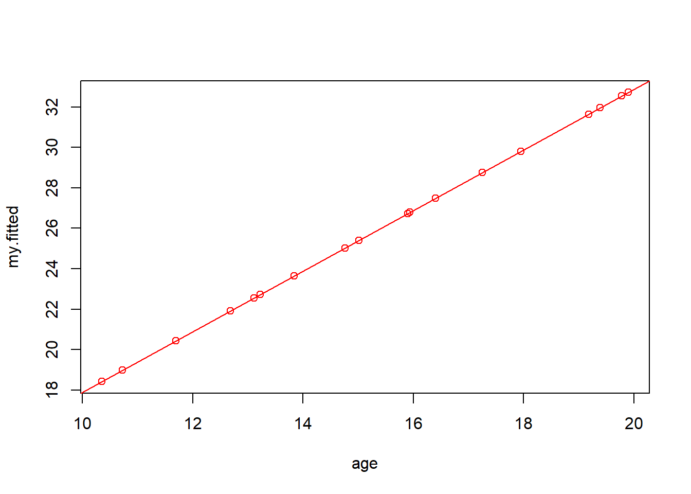

Alternatively, instead of calculating these “by hand”, I could simply extract the fitted values directly from the model results using:

my.lm$fitted.values

##         1         2         3         4         5         6         7         8 
## -1.849460 -1.849460  9.947766  9.947766 13.880175 17.812584 21.744993 21.744993 
##         9        10        11        12        13        14        15        16 
## 21.744993 25.677401 25.677401 29.609810 29.609810 29.609810 29.609810 33.542219 
##        17        18        19        20        21        22        23        24 
## 33.542219 33.542219 33.542219 37.474628 37.474628 37.474628 37.474628 41.407036 
##        25        26        27        28        29        30        31        32 
## 41.407036 41.407036 45.339445 45.339445 49.271854 49.271854 49.271854 53.204263 
##        33        34        35        36        37        38        39        40 
## 53.204263 53.204263 53.204263 57.136672 57.136672 57.136672 61.069080 61.069080 
##        41        42        43        44        45        46        47        48 
## 61.069080 61.069080 61.069080 68.933898 72.866307 76.798715 76.798715 76.798715 
##        49        50 
## 76.798715 80.731124

Again, the important takeaway here is the fitted values are those that correspond to the \(x\) values which fall right along our regression line.

18.4.7 Residuals

So now we’re in a a position to start to understand the uncertainty that exists in our model. Referring to the previous graph, we recognize that our original data didn’t fall so neatly on the graph. How far off were they and can we quantify this difference? Yes, we can!

Referring again back to our model, we had: Data (\(y\)) = Fitted (\(\beta_0 + \beta_1 x\)) + Residual (\(\epsilon\)). So then, what are the residuals?

I’ll attempt to describe this both visually and using algebra.

First, our residuals are the data minus fitted, so let’s plot both our data and fitted results on the same plot. The plot below shows the original data points, \(y_i\), in black and the fitted values, \(\hat y_i\), (for each x) in red:

plot(age, my.fitted, col="red", ylim=c(15, 35), ylab="strength")
points(age, strength)   # the points() function adds points to an existing plot
legend(10.25, 35, c("data", "fitted"), col=c("black", "red"), pch=1)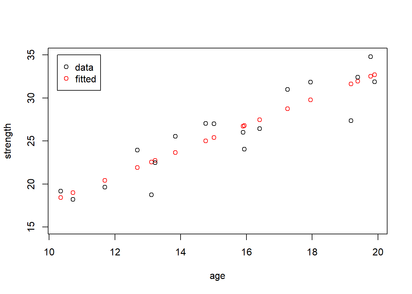

The red points of course fall on the fitted line, and the black points are all either above or below their corresponding fitted value. But this plot is admittedly a little difficult to interpret.

So, let’s add the residuals. I’ll draw blue line segments to show the length (size) of each residual:

plot(age, my.fitted, col="red", ylim=c(15, 35), ylab="strength")
points(age, strength)
segments(age, strength, age, my.fitted, col="blue")
legend(10.25, 35, c("data", "fitted"), col=c("black", "red"), pch=1)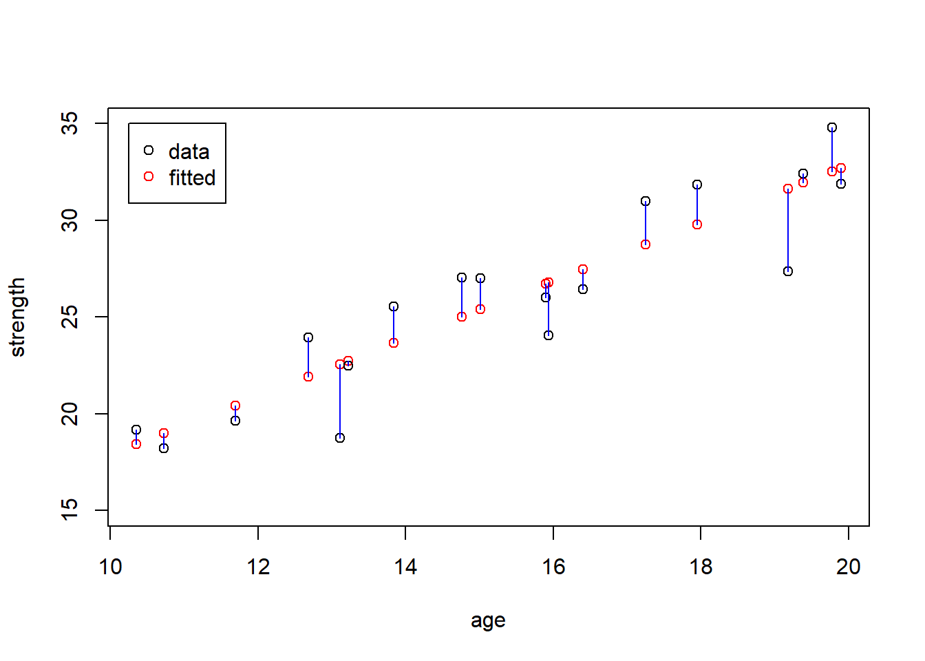

Here’s it’s easier to see how each original data point and its fitted value correspond. And note that the \(x\) value is the same for each pair of data and fitted, it’s the \(y\) value that changes. As a reminder, the intent of this is to illustrates that:

Data (\(y\), black) = Fitted (\(\beta_0 + \beta_1 x\), red) + Residual (\(\epsilon\), blue)

Some notes:

• residuals can be positive or negative, depending on whether the original data is above or below the fitted value,
• residuals are the vertical distance between the fitted and observed data. Using the vertical distance makes the most sense when thinking about “prediction”
• the residuals should sum to zero, which is an outcome of how we create our best fitting line

Similar to our fitted values, we can quickly calculate the residuals by vector math particularly once we have our fitted values:

strength-my.fitted

##  [1]  0.466426 -0.768052  0.735690  2.262752 -2.750304  2.031530 -0.740440
##  [8] -0.826840  1.601534 -0.249552 -0.799754 -1.038740  1.912556  2.005684
## [15]  2.018612 -3.814926  2.229150 -4.289288

or simply extract these from our model by using:

str_age.lm$residuals

##          1          2          3          4          5          6          7 
##  0.4674031 -0.7675119  0.7362115  2.2637488 -2.7495008  2.0324346 -0.7396388 
##          8          9         10         11         12         13         14 
## -0.8258372  1.6022904 -0.2488858 -0.7991650 -1.0379136  1.9132534  2.0064278 
##         15         16         17         18 
##  2.0192509 -3.8142654  2.2300193 -4.2883214

Again within rounding, these two approaches yield similar results.

Additionally, for the last bullet point we see:

sum(str_age.lm$residuals)

## [1] 8.326673e-16

which should be exactly 0, but is an effect of R’s rounding algorithm. Assuming our best fitting line goes through the point \(\bar x, \bar y\) (which it does), the residuals will sum to zero.

18.4.8 Guided Practice

Find the fitted values and the residuals for relationship between speed and braking distance in the cars data.

18.4.9 Our Best Fitting Line

Now we’re in a position to describe why we choose the specific regression line we do.

You may have heard the term “Least Squares Regression”. Our regression line is going to minimize the sum of squares of the residuals. As a reminder, we discussed sum of squares quite a bit during our ANOVA chapter, and it is the key component of our variance calculations.

As was shown above, the residuals depend on the fitted values and therefore on the specific regression line. For the same set of observed data, different fitted lines (different values of \(\beta_0\) and \(\beta_1\)) will result in different fitted points. Above we used my.fitted <- 1.4966*age+2.9345, but what if we used slightly different numbers for \(\beta_0\) and \(\beta_1\)? That would result in different fitted results and therefore different residuals. So, how do we decide what’s best?

In summary, we’ll choose values of \(\beta_0\) and \(\beta_1\) that minimize \(\sum\epsilon_i^2\) (hence “least squares”).

The section below is optional, and describes the math (calculus) about why/how the values we chose accomplish this.

18.4.10 Optional: Summary of the math behind the coefficients

In a higher level statistics class you would learn the mathematics (including calculus) behind how we determine the best fitting line that minimizes the least square error. (i.e. what and why are the equations for the coefficients of best fitting line.)

To give a quick overview, our sum of squares residuals (SSR) are:

\[\sum (Y_i-(X_i*\beta_1+\beta_0))^2\]

and our goal is to find the values of \(\beta_0\) and \(\beta_1\) that minimize this expression.

To do that we would take the partial derivative of this with respect to each of our coefficients and set each of the resulting equation to zero. Then, we’d have two equations and we could solve these simultaneously to find the values of \(\beta_0\) and \(\beta_1\).

In terms of the results, if we define the sum of squares of the \(x\) as \(ss_{x} = \sum(x_i-\bar x)^2\) and the sum of squares of the \(xy\) as \(ss_{xy} = \sum(x_i-\bar x)(y_i-\bar y)\), then \(\beta_1 = \frac{ss_{xy}}{ss_{x}}\) and \(\beta_0 = \bar y - \beta_1 \bar x\).

A good description of the the details of the math is available from Wolfram: https://mathworld.wolfram.com/LeastSquaresFitting.html.

18.4.11 Optional: Connecting \(\beta_1\) and \(r\)

Interestingly, our best fitting slope parameter \(\beta_1\) is also related to our correlation, \(r\).

It turns out that \[\beta_1 = \frac{s_y}{s_x}*r\] where \(s_x\) and \(s_y\) are the standard deviations and \(r\) is the correlation. So from above we found \(\beta_1 = 1.4966\) and here:

sd(strength)/sd(age)*cor(age, strength)

## [1] 1.49655

I won’t ask you to do this, I simply wanted to point out the link between correlation and our slope parameter.

And from there, because the best fitting line goes through the means of both data sets, (why?) we can easily find \(\beta_0 = \bar y - \beta_1\bar x\).

mean(strength)-1.4966*mean(age)

## [1] 2.933724

Why is the point (\(\bar x, \bar y\)) is on our line?

18.4.12 What about other lines?

Q: What would be wrong if we just picked the first and last data points and put a line through those?

A: Yes, certainly there are a number of others ways we might choose a line, but those other approaches aren’t guaranteed to minimize the (sum of square of the) residuals. That will lead to more uncertainty in our model, and make prediction worse.

18.4.13 Plotting the residuals

In addition to being useful to determine the best fitting line, analysis of residuals helps us answer two important questions:

1. is a linear model appropriate?
2. how much uncertainty exists?

We’ll get to the second point in a different section, and here, as our last step in “fitting” our model, we will use the residuals to evaluate whether a linear model is really appropriate.

One way to do this is using a plot of residuals, as a function of \(x\). The reason to do this is we want to see if the residuals are random, or if there’s any trend in them, particularly as \(x\) increases. Here is the residual plot for the age vs. strength data, and note I am plotting these as a function of \(x\) (age).

plot(age, str_age.lm$residuals, ylab="residual value")
abline(h=0, col="red", lty=2)

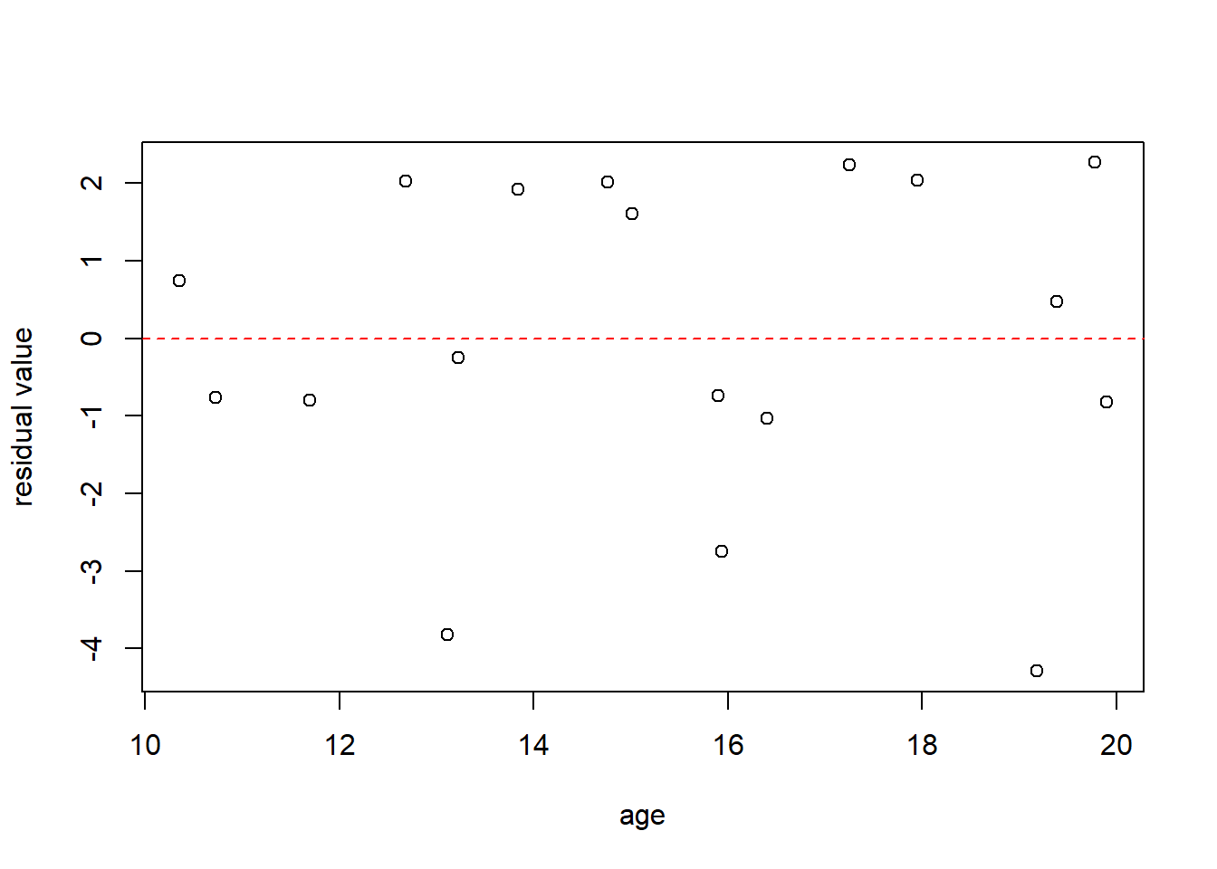
What do we see? Note I’ve added a horizontal line at \(y=0\), because we expect them to be centered around that value. Remember, the residuals sum to zero, and this itself is NOT an indication of a good fit.

Questions you might ask of the above plot include:

• Is there any obvious trend in the residuals as a function of \(x\)?
• Are there equal numbers of residuals above and below the dashed line?
  
• Are the residuals mostly centered near 0, with fewer appearing farther away?
• Is the variation in the residuals seem constant as a function of \(x\)? Or does the spread of the residuals away from the dashed line (in the vertical direction) increase or decrease as \(x\) changes?

I’d be slightly worried about the three larger negative residuals here.

Additionally, above we said that residuals should have a Normal distribution. What does that mean exactly? Let’s also look at a histogram of the residuals:

hist(str_age.lm$residuals, main="Histogram of residuals", xlab="residual value")

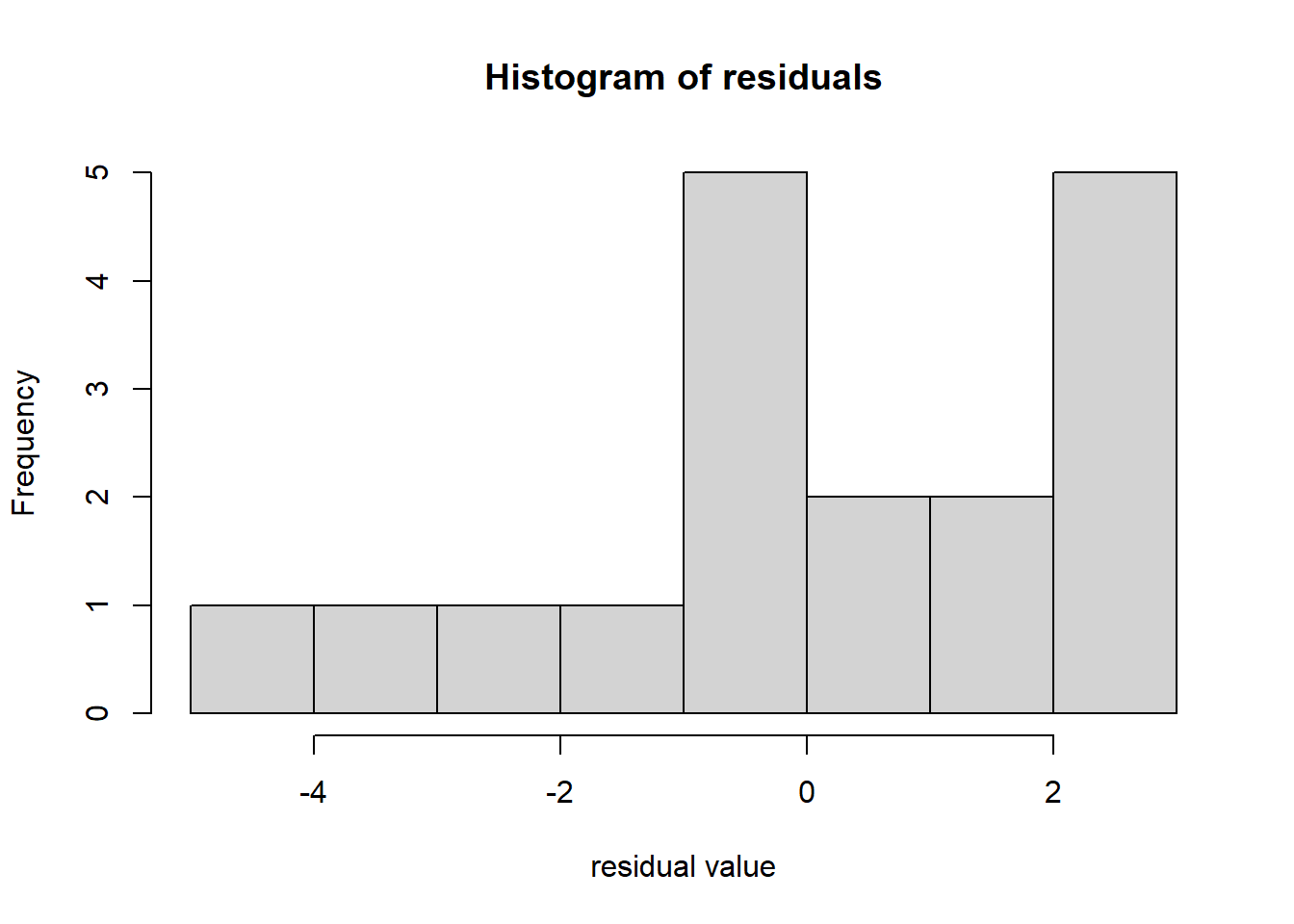
Does this appear to be a Normal distribution centered around 0? Not really! But as we saw above in an earlier chapter, simulating small samples from a Normal distribution can be deceiving.

There are other, more advanced techniques to evaluate residuals, but those are beyond the scope of this class. The important takeaway here is that we want the residuals of our fitted model to be without bias and randomly distributed. This is important both for evaluating whether a linear model is appropriate AND to ensure that we limit any bias in our predictions.

18.4.14 Visualizing the Uncertainty in the Residuals

The following image is attempting to show is that each fitted value (the point on the line) is in fact the mean of a distribution that is roughly “Normal”.

The plot below shows our age vs. strength data, where the red distribution curves in the plot should be interpreted as being in the \(z\)-dimension, i.e. coming off the page.

Since our \(\epsilon\) have a Normal distribution, in fact there’s really a Normal distribution at each \(x\) value, and hence uncertainty about where observed data will fall.

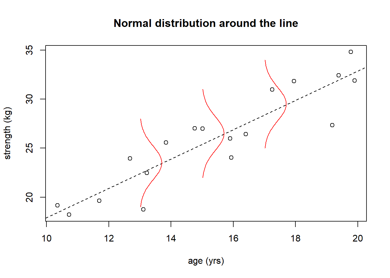
The three \(x\) values are chosen to be illustrative, and in fact the normal distribution extends the length of the fitted line.

18.4.15 What would bias or trend in residuals look like?

The following is simulated data that is intentionally not linear. Notice the \((x_2)^4\) term. It generally looks linear, but if you inspect it closely, you might notice the curve upwards as \(x\) increases.

n <- 25
x2 <- runif(25, 2, 20)
y2 <- 0.5*x2^2+4 + rnorm(25, 0, 5)
plot(x2,y2)

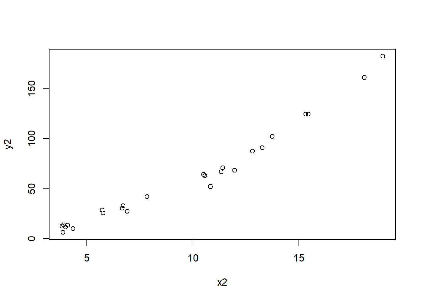
Ignoring that for the moment, let’s fit a linear model and plot the trend line:

my.lm2 <- lm(y2~x2)
plot(x2, y2)
abline(my.lm2, col="red")

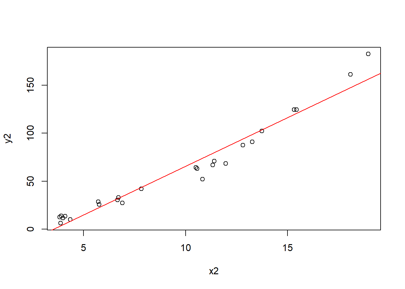
Here we might start to suspect a problem with our model. What’s happening to the data points with respect to the fitted line?

Next, plot the residuals as a function of \(x_2\).

plot(x2, my.lm2$residuals)
abline(h=0, col="red", lty=2)

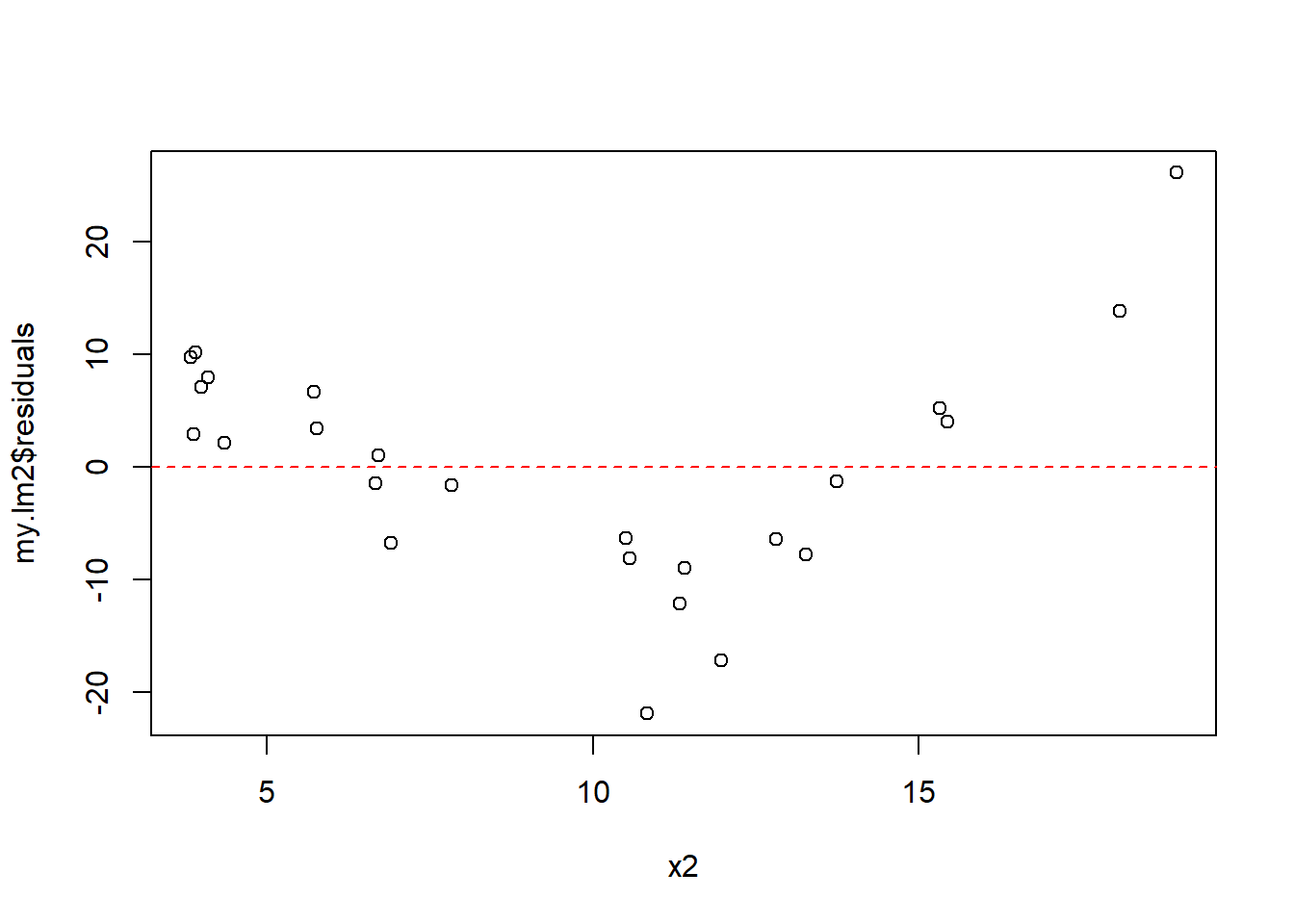
What do you notice about the distribution of these residuals? Do they appear randomly distributed about the \(y=0\) line? Obviously not!

Our first questions from above was: Is there any obvious trend in the residuals as a function of \(x\)? Here the answer is “yes”.

Particularly with respect the first question, we see that the residuals for \(x<7\) are all above the \(y=0\) line, then for \(7<x<15\) values of all the residuals are below the line, and finally, for \(x>15\) are all above the line. This is an obvious trend, and means that a linear model would be invalid.

18.4.16 Summary and Review

That concludes our discussion of the fitted model, the best fitting (“least squares”) line, and analysis of the residuals to evaluate model fit.

Based on this section you should now be able to:

• Fit a linear model using the lm() function in R and extract the slope and intercepts coefficients of the best fitting line.
• Understand what is meant by “best fitting line” and “least squares regression”, namely that these lines minimize the sum of squared residuals, \(\sum \epsilon_i^2\)
• Interpret the slope and intercept coefficients in terms of the original data
• Overlay the fitted line onto a scatter plot of the data
• Define the terms “observed data”, “fitted data” and “residuals”, and both describe how they relate to our “model” as well as how they relate to one another
• Calculate or extract the residuals and plot them to evaluate if the assumptions of no bias or trend, random distribution and constant variance seems reasonable

18.5 Statistical Analysis of the Fitted Line

Now that we know how to fit a linear model, we’ll dive deeper into the statistical analysis to explore the uncertainty that exists in our model. One of main goals here is to understand if the relationship exists between our predictor and response variables. Also, we’ve said the residuals comprise the error and have a Normal distribution. What are the implications of this?

After this section, you should be able to:

• Discuss why we test \(H_0: \beta_1=0\) to see if there is a “significant” relationship between \(x\) and \(y\)
• Describe why is there uncertainty around our coefficients, and explain the difference between \(\beta_1\) and \(\hat \beta_1\)
• Interpret the summary() output for a linear model
• Determine a 95% confidence interval on \(\beta_1\) and explain how that interval relates to \(H_0\)
• Extract the \(R^2\) value from our model and explain how it informs to model fit

18.5.1 A Statistically Significant Relationship between \(x\) and \(y\)

Above we showed how to estimate the values of the slope (\(\beta_1\)) and intercept (\(\beta_0\)) parameters, but does that necessarily mean that a linear relationship exists? In short, no, and in this section we’ll learn how to evaluate this.

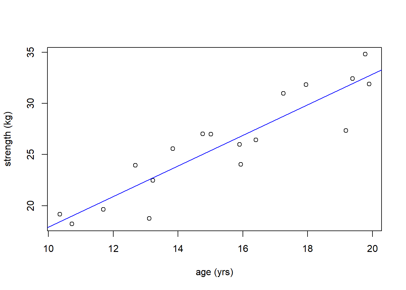
Again here we’ll use our strength vs. age data with the fitted line, shown in the plot below:

plot(age, strength, xlab="age (yrs)", ylab="strength (kg)")
abline(str_age.lm, col="red")

Is there a “statistically significant” relationship between age and strength? And what do we mean by that?

So based on the above plot you’d probably say there’s a strong positive linear relationship between \(x\) (age) and \(y\) (strength). Next, let’s extract the values of the coefficients:

str_age.lm$coefficients

## (Intercept)         age 
##     2.93450     1.49655

Which tells us for every unit increase in \(x\) (age) i.e. every year, \(y\) (strength) increases on average by 1.496 units (kg).

However, looking at the raw data, as we said, it’s a fairly strong relationship. Would you have been surprised if the best fitted line were perfectly horizontal (i.e. \(\beta_1 = 0\))? Probably so.

This is an important point. If the slope were 0, the best fitting line would be a horizontal line. In that case, \(x\) would NOT be a good predictor of \(y\). Knowing a value of \(x\) wouldn’t tell us anything useful about the corresponding value of \(y\). So, to determine if there is a “statistically significant” relationship between \(x\) and \(y\), we’re going to evaluate if the slope parameter is statistically different than 0.

The inherent null hypothesis is running a regression analysis is \(H_0: \beta_1 = 0\) with an alternative hypothesis of \(H_0: \beta_1 \ne 0\).

Importantly, just because we can fit a line to some data and estimate \(\beta_1\), it does NOT necessarily mean that a statistically significant relationship exists. We’ll need to dive deeper into the uncertainty to determine that.

18.5.2 Using the summary() Output

Let’s look at the linear model results for the above strength vs. age data, using the summary() command (similar to what we did with ANOVA):

summary(str_age.lm)

## 
## Call:
## lm(formula = strength ~ age)
## 
## Residuals:
##     Min      1Q  Median      3Q     Max 
## -4.2883 -0.8192  0.1093  1.9831  2.2637 
## 
## Coefficients:
##             Estimate Std. Error t value Pr(>|t|)    
## (Intercept)   2.9345     2.6340   1.114    0.282    
## age           1.4965     0.1679   8.911 1.33e-07 ***
## ---
## Signif. codes:  0 '***' 0.001 '**' 0.01 '*' 0.05 '.' 0.1 ' ' 1
## 
## Residual standard error: 2.142 on 16 degrees of freedom
## Multiple R-squared:  0.8323, Adjusted R-squared:  0.8218 
## F-statistic:  79.4 on 1 and 16 DF,  p-value: 1.333e-07

Yes, this is quite long! There are a couple of interesting things in this result I’d like you to focus on:

• The coefficients table is given in lines 9-12 of the output. Here we see \(\beta_0 = 2.9345\) and \(\beta_1 = 1.4965\), matching our above results
• The overall p-value listed on the last line of the output is 1.33e-07, and so since our null hypothesis here is that \(\beta_1 = 0\), we would reject \(H_0\) and conclude that the slope coefficient is significantly different than zero.

Ponder these questions:

\(Q_1\): Why does evaluating \(\beta_1=0\) relate to whether there is a statistically significant relationship between \(x\) and \(y\)?
\(Q_2\): What if the slope was 0? What would that mean?

\(A\): If the fitted slope were 0, then as \(x\) increases, we wouldn’t expect \(y\) to change, particularly not the average value of \(y\). (However, because of the uncertainty that exists, of course, individual values might increase or decrease.) So, if there’s NO relationship between the variables, then we don’t expect that knowing \(x\) will help us predict what \(y\) is.

But how did we find the p-value? This is simply the result of a t-test, based on the standard error. But why is there uncertainty in our estimates coefficient values? We will tackle that shortly.

18.5.3 Guided Practice

The following data (not real) shows the relationship between annual rainfall in Seattle and the price of gas between 1980 and 2019:

rain <- c(36.5, 38.9, 37.4, 29.0, 37.5, 43.3, 36.3, 30.3, 32.9, 39.7, 36.1, 43.2, 35.8, 40.7, 39.8, 47.2, 45.2, 33.6, 45.5, 37.9, 35.7, 44.1, 37.3, 40.8, 41.3, 44.7, 40.6, 46.4, 33.9, 38.1, 34.9, 47.2, 38.6, 42.1, 31.8, 31.0, 35.8, 34.9, 45.1, 35.7)
gas <- c(1.58, 1.51, 1.46, 1.48, 1.49, 1.79, 1.83, 1.70, 1.69, 1.72, 1.86, 1.36, 1.78, 2.55, 1.89, 2.56, 2.68, 2.09, 2.32, 1.99, 2.03, 2.34, 2.35, 2.15, 2.27, 3.08, 2.78, 3.16, 2.83, 3.05, 2.91, 3.38, 2.86, 3.00, 3.62, 3.56, 3.58, 3.47, 3.51, 3.39)
plot(rain, gas, xlab="annual rainfall (in)", ylab="gas prices ($/gallon)")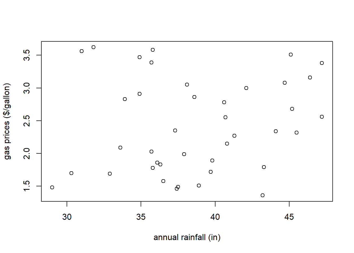

• What do you observe about the relationship? Describe what you see in the scatter plot. What type of relationship would you expect between these variables?
  
• Fit a linear model to the data
• Add the fitted line to the plot. What do you now observe?
• Output the summary() of the linear model including the coefficients and p-value. Does it seem that there is a statistically significant relationship between annual rainfall and gas prices?

18.5.4 Why is there Uncertainty in our Coefficients?

So you may be a little confused at this point. We’ve estimated a non-zero value of \(\beta_1\) yet we’re saying we want to evaluate if it’s “statistically” different than 0. What does that mean? And why is there uncertainty in our estimates anyway?

I’ll describe this two ways: first related to our assumptions and the second related to our model. The second is admittedly bit more technical and hence included in the optional sections below.

At the highest level, one of the assumptions we’re making when we perform statistical regression analysis is that we are merely taking a sample of data from a larger population. Our sample is hopefully representative, but incomplete. This is similar to assumptions we made in earlier chapters when making inference about 1 or 2 samples.

The implication of this is that if we were to take a different sample, even at the same \(x\) values, we would potentially see different \(y\) values. This is a key point, make sure it is clear. Then, if we were to then fit a regression model to this new data, we would potentially see different coefficient values, i.e. a different fitted line.

This is analogous to work we did earlier calculating \(\hat p\) or \(\bar x\), where we were knew there was uncertainty in estimating \(p\) or \(\mu\). Again here, if we took a different sample, our calculated values would change slightly.

To distinguish between the sample and the population values in regression, let’s introduce the ideas of \(\hat \beta_0\) and \(\hat \beta_1\) as our parameter estimates to distinguish these from \(\beta_0\) and \(\beta_1\), the true population values.

So yes, our value of \(\hat \beta_0\) and \(\hat \beta_1\) are the best estimates of \(\beta_0\) and \(\beta_1\) based off our sample data. Again, they are most likely different because were we were to take a different sample, we’d likely calculate different values of \(\hat \beta_0\) and \(\hat \beta_1\). This is what we mean about uncertainty in our coefficients, in that applies not to our specific sample, but to the inference we make to the larger population, and the true values of \(\beta_0\) and \(\beta_1\).

18.5.5 Optional: Independence of Residuals

The second reason for uncertainty in our coefficient estimates goes back to our “model”, which assumes that the residuals \(\epsilon_i\) are random and independent of the \(x\) value.

As mentioned above, were we to go take another sample of our data, at the same \(x\) values, we would expect to see different \(y\) values. If our model is correct, those different \(y\) values would result not from different coefficient values, but different residuals, since those are assumed to be random. Each observed value is the result of the fitted line + the error, and every time we sample a different point, our error is a random variable with a \(N(0, \epsilon)\) distribution.

Yet, since we only observe the original data values, the mixing around of residuals would likely result in a different best fitting line.

And once we assume the residuals are random and could have (in a different sample, for example) been just as likely attached to other points, we realize the observed line is just one of many possibilities within the population.

Therefore there is uncertainty around our best fitting line (and the coefficients of it).

Importantly, just like we previously used standard error to estimate the uncertainty in \(\hat p\) or \(\bar x\), here we can use the residuals to estimate the uncertainty in \(\beta_0\) and \(\beta_1\).

Hence, one of our goals in regression analysis is to make inference about the true value of \(\beta_1\), not simply relying on our observed sample value, \(\hat \beta_1\).

18.5.6 Using the summary() Output for Hypothesis Testing

So, armed with an understanding of why there’s uncertainty in our parameter estimates, we can proceed to evaluate what the implications are. As we’ll see, our approach will generally follow our hypothesis testing from previous chapters.

Here again is the summary output of our fitted model:

summary(str_age.lm)

## 
## Call:
## lm(formula = strength ~ age)
## 
## Residuals:
##     Min      1Q  Median      3Q     Max 
## -4.2883 -0.8192  0.1093  1.9831  2.2637 
## 
## Coefficients:
##             Estimate Std. Error t value Pr(>|t|)    
## (Intercept)   2.9345     2.6340   1.114    0.282    
## age           1.4965     0.1679   8.911 1.33e-07 ***
## ---
## Signif. codes:  0 '***' 0.001 '**' 0.01 '*' 0.05 '.' 0.1 ' ' 1
## 
## Residual standard error: 2.142 on 16 degrees of freedom
## Multiple R-squared:  0.8323, Adjusted R-squared:  0.8218 
## F-statistic:  79.4 on 1 and 16 DF,  p-value: 1.333e-07

What’s critical here is the table within the ## Coefficients: section. The first row of the table represents the intercept and the second row represents the slope. The columns contain information about: the Estimate (the point estimate), the Std.Error (the standard error), the t value (the test statistic) and Pr(>|t|) (the p-value).

Before we dive too deeply into all of that, let’s get in our WABAC (https://rockyandbullwinkle.fandom.com/wiki/WABAC_machine) machine. Haha.

In Winter trimester, for small samples with \(\sigma\) unknown, we used a t-distribution, AND if we wanted to know if the mean was different than 0, we found our test statistic as \[t_{df}\sim \frac{\bar X}{SE}\]

We then compared this value against a \(t\) distribution with the appropriate degrees of freedom. We will take the same approach here.

In particular, if we look at \(\beta_1\), the estimate is 1.4965 with a standard error of 0.1679, so the corresponding test statistic is \(\frac{1.4965}{0.1679} = 8.911\).

And note that, we can use this test statistic to find our p-value as based on a t-distribution with 16 degrees of freedom. Why is \(df=16\)? There were \(n=18\) data points in our original data, and for simple linear regression (with one predictor variable) \(df = n-2\).

Let’s draw the picture of this t-distribution just to remind ourselves what this represents:

xt <- seq(from=-3, to=3, by=0.05)
yt <- dt(xt, 16)
plot(xt, yt, type="l", main="t Distribution with df=16")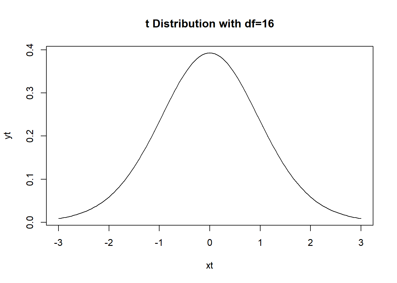

Of course, a test statistic value of \(8.911\) is so extreme it doesn’t even show on this plot. Hence the extremely small p-value.

So what’s the probability of seeing a value as extreme as \(8.911\)? This is a two-sided test because we reject \(H_0\) if the slope was either too small (negative) or too large (positive). In either case we would consider it to be “different than 0”. For our test statistic we find the p-value as:

2*pt(8.911, 16, lower.tail=F)

## [1] 1.332202e-07

and since this is much, much smaller than \(\alpha=0.05\), we’d reject our null hypothesis and conclude that the slope parameter \(\beta_1\) is significantly different than 0.

What’s important to remember is that if \(\beta_1\) is not significantly different than 0, then it has no predictive value, meaning using it in our model is pretty useless. We’d be better off just using the mean \(\bar y\) as the best estimate of \(y\).

18.5.7 Optional: Estimating \(\epsilon\)

As a reminder, our model is \(y = \beta_0 + \beta_1 x + \epsilon\) and we assume the residuals have a \(N(0, \sigma_\epsilon)\) distribution.

How do we estimate \(\sigma_\epsilon\)? This is NOT the standard error. Here’s our summary output:

summary(str_age.lm)

## 
## Call:
## lm(formula = strength ~ age)
## 
## Residuals:
##     Min      1Q  Median      3Q     Max 
## -4.2883 -0.8192  0.1093  1.9831  2.2637 
## 
## Coefficients:
##             Estimate Std. Error t value Pr(>|t|)    
## (Intercept)   2.9345     2.6340   1.114    0.282    
## age           1.4965     0.1679   8.911 1.33e-07 ***
## ---
## Signif. codes:  0 '***' 0.001 '**' 0.01 '*' 0.05 '.' 0.1 ' ' 1
## 
## Residual standard error: 2.142 on 16 degrees of freedom
## Multiple R-squared:  0.8323, Adjusted R-squared:  0.8218 
## F-statistic:  79.4 on 1 and 16 DF,  p-value: 1.333e-07

Looking at the lower part of the output (line 16) we see: Residual standard error: 2.142. Where does this come from? The equation for \(\sigma_\epsilon\) is \[\sqrt{\frac{1}{n-2}\sum \epsilon_i^2}\]

Calculating this by hand we find:

sqrt(sum(str_age.lm$residuals^2)/str_age.lm$df.residual)

## [1] 2.142048

Why \(n-2\)? (And why is this our degrees of freedom?) Because we’re estimating \(\beta_0\) and \(\beta_1\) so we only have \(n-2\) degrees of freedom left. We saw this above with our t-distribution.

Hence, when we say that the residuals \(\sim N(0, \sigma_\epsilon)\), the Residual Standard error is our best estimate of \(\sigma_\epsilon\), the standard deviation of the residuals.

18.5.8 Confidence Intervals on \(\beta_0\) and \(\beta_1\)

Since we’re now familiar with the uncertainty around \(\beta_0\) and \(\beta_1\), what about confidence intervals on where the true values lie?

Let’s focus again on the Coefficients: table. Since we know each coefficient’s estimate and standard error, and we can use these to find the likely range of the true value of each. Again, this is analogous to using \(\bar X\) and SE to find the confidence interval on true value of \(\mu\).

Our \(\alpha\) level confidence interval the true value of \(\beta_1\) will be

\[\hat \beta_1 \pm t_{df, \alpha}*SE_{\beta_1}\]

which is similar to “mean plus or minus 1.96 times the standard error”, but here we’re using coefficient estimate \(\hat \beta_1\), the appropriate t-distribution multiplier (2.12) and the estimated standard error for \(\hat \beta_1\). So specifically in this case we’d calculate a 95% confidence interval on the true value of \(\beta_1\) as:

1.4965 - qt(0.975, 16)*0.1679

## [1] 1.140568

1.4965 + qt(0.975, 16)*0.1679

## [1] 1.852432

Also note that I’ve called our estimate of the slope \(\hat \beta_1\). This is technically more correct.

What does this interval mean? Remember, it’s a confidence interval. So, if we ran this experiment 100 times, collecting data each time and estimating \(\beta_1\) and it’s standard error, the true value of \(\beta_1\) would lie within 95 of those calculated intervals.

And, this is probably obvious, but if our 95% confidence interval contains the value of zero, its highly likely that we will fail to reject \(H_0\) at \(\alpha=0.05\). This is not the case here.

18.5.9 Guided Practice

• Using the cars dataset, is speed a statistically significant predictor of braking speed? What is a 95% confidence interval on the true value of \(\beta_1\)?

• Using the rainfall vs. gas usage dataset from above, What is a 95% confidence interval on the true value of \(\beta_1\)?

18.5.10 Optional: Calculating the Standard Error on \(\beta_0\) and \(\beta_1\)

Above we saw that R outputs the standard error values for \(\beta_0\) and \(\beta_1\), which we used to test their significance. Where do those values come from?

Deriving these is beyond the scope of this class, so suffice it to say that they are a function of the \(\epsilon_i^2\) and data themselves.

18.5.11 What is \(R^2\)?

There is one other important statistic included in the summary table that helps us answer the question: “how good is our model?”: the \(R^2\) value.

Although this won’t answer how good of a fit a linear model is to our data, it is helpful to tell us “how useful of a predictor do we have?” \(R^2\) compares the overall variance in the original response (\(y\)) data to the variance of the residuals. You can think about the residual variance as the amount that is “left over” after fitting the model.

A good model will “explain” almost all of the variation we see.

Let’s start by looking at how much variation there is in the response variable, \(y\). Calculating that is fairly straightforward:

var(strength)

## [1] 25.74909

By itself, this is somewhat of a meaningless quantity.

What we really care about, is how much variation is left (i.e. still unexplained) after including the predictor in the model? Ideally, a perfect model would explain 100% of the variation (so 0% left) whereas a horrible model would explain almost none of the variation (so near 100% left.)

The variation left is simply the variation in the residuals. We can find this as:

var(str_age.lm$residuals)

## [1] 4.318465

We see that this is a much smaller value. And maybe an easier way to interpret this is by calculating the percent of the variation in \(y\) is explained by having \(x\) in the model. We’ll do this as:

resid.var <- var(str_age.lm$residuals)
resp.var <- var(strength)

(resp.var - resid.var)/resp.var

## [1] 0.8322867

Conveniently, in the above table, you’ll see an output titled “Multiple R-squared: 0.8323” which matches our calculation here.

What this means is that our linear model (i.e. the one that includes age as a predictor) explains 83.2% of the original variation in \(y\). This is a pretty good model!

One of the main goals of (linear) regression analysis is to attempt to explain the variation we see in \(y\). If we could explain away all of the variation, that would be fantastic, and certainly quite useful for both understanding the system and making predictions. So, the \(R^2\) value is a measure of how much of that observed variation that we can explain.

18.5.12 The Relationship between \(r\) and \(R^2\)

We previously used the correlation, \(r\), to assess the strength of the linear relationship. The \(R^2\) value here is exactly that, namely the square of the correlation:

cat("correlation:", cor(age,strength), "\n")
cat("R-squared  :", cor(age,strength)^2, "\n")

## correlation: 0.9122975 
## R-squared  : 0.8322867

And since \(-1 \le r \le 1\), it must be the case that \(0\le R^2 \le 1\).

So again, similar to how correlation doesn’t tell us about a “linear” fit, a high \(R^2\) value doesn’t necessarily mean the relationship is linear.

18.5.13 Summary and Review

In this section we discussed hypothesis testing for linear regression with a focus on attempting to understand if \(\beta_1=0\) because this tells us if \(x\) is a useful predictor.

Based on this section, you should now be able to:

• Discuss why we test \(H_0: \beta_1=0\) to see if there is a “significant” relationship between \(x\) and \(y\)
• Describe why is there uncertainty around our coefficients, and explain the difference between \(\beta_1\) and \(\hat \beta_1\)
• Interpret the summary() output for a linear model
• Determine a 95% confidence interval on \(\beta_1\) and explain how that interval relates to \(H_0\)
• Extract the \(R^2\) value from our model and explain how it relates to model fit

18.6 Using our Fitted Line for Prediction

In the previous section we discussed the concept of why there is uncertainty in our estimates of \(\beta_0\) and \(\beta_1\). More formally, we would write the true population value for the slope as \(\beta_1\) and our estimated value based on our sample as \(\hat \beta_1\). As a reminder, one of our main goals in regression analysis specifically (and statistical analysis in general) is to use our observed (sample) data to make inference about the population.

Hence, our next “big” topic for regression is to understand the idea of how we might use our fitted model for prediction.

What in particular might that mean? Generally it means predicting the \(y\) (response) value we might see for a given (or new) \(x\) (predictor) value. And while it’s worth noting that we could simply plug in the new \(x\) value into our fitted equation to find a point estimate, doing so doesn’t incorporate the uncertainty we know exists.

So the first point here is that when we discuss prediction, we’re talking about the range of likely \(y\) values we might see for a given \(x\).

Further, there are generally two types of prediction we might make. For a given \(x\) value we might predict the range of:

• the average response
• an individual response

With a little thought, you can probably recognize that the range of the first will be narrower than that of the second.

We’ll calculate both of these using a type of confidence interval, and to do so, we’ll use values a new function in R, predict().

18.6.1 Learning Objectives

Based on this section, you should be able to:

• Discuss why a point estimate is really insufficient when making a prediction
• Explain the different types of intervals we might calculate for prediction of a new result, including:
  • Where the average result might fall, (the so-called “confidence interval of the prediction”), and
    
  • Where any individual result might fall, (the “prediction interval”)
    
• Explain why there is more uncertainty in predicting the range of any individual value compared with the range of the average value
• Describe why the average predicted value and the range of regression lines are the same
• Use the predict(..., interval="confidence") function to calculate a 95% confidence interval on where the mean value of \(y\) will fall for a given value of \(x\).
• Use the predict(..., interval="prediction") function to calculate a 95% prediction interval describing the likely range of where a single value of \(y\) might occur for a given value of \(x\).
• Explain why it is inappropriate to make a prediction using an \(x\) value that’s outside of the range of our observed \(x\) data

18.6.2 Using the predict() Function to Find the Average Result

Conceptually, here’s what we’re doing: We know there is uncertainty in \(\beta_0\) and \(\beta_1\), so here we’re looking at the likely range where the best fitting regression line might fall.

In R, we’ll use the predict() function, and to do this, the first thing we need to do is figure out the x value where we want to make the new prediction. Let’s call that \(x^*\).

Going back to our strength vs. age data, repeated here for ease of access:

plot(age, strength, xlab="age (yrs)", ylab="strength (kg)")
abline(str_age.lm, col="blue1")

What would the likely average range of strength be for a 17 year old? I will first show you how to do this using predict(), then revisit the theory of why and where this uncertainty exists. Remember, our goal here is not to just simply find the value on the fitted line, but the range of possible values.

As a first step to using the predict() function, we need to create a new dataframe with the appropriate column name. The column name needs to match our original data set.

newx <- data.frame(age = c(17))

We then call the predict() function, using our model and this newx variable, and we tell R the “type” of prediction we’re trying to make. What we’re doing here is known as a confidence interval of the prediction so we’ll use interval ="confidence".

predict(str_age.lm, newdata = newx, interval="confidence")

##        fit      lwr      upr
## 1 28.37584 27.16217 29.58952

What this shows us is that the likely range (in fact the 95% confidence interval) on the average value of strength if age = 17 is somewhere between {27.16, 29.59}. The fit refers to the value on the line at \(x=17\).

The red segment in the plot below shows the range of predicted values at \(x=17\).

plot(age, strength, xlab="age (yrs)", ylab="strength (kg)")
abline(str_age.lm, col="blue1")
segments(17, 27.16, 17, 29.59, col="red")
points(c(17, 17), c(27.16, 29.59), pch=20, col="red")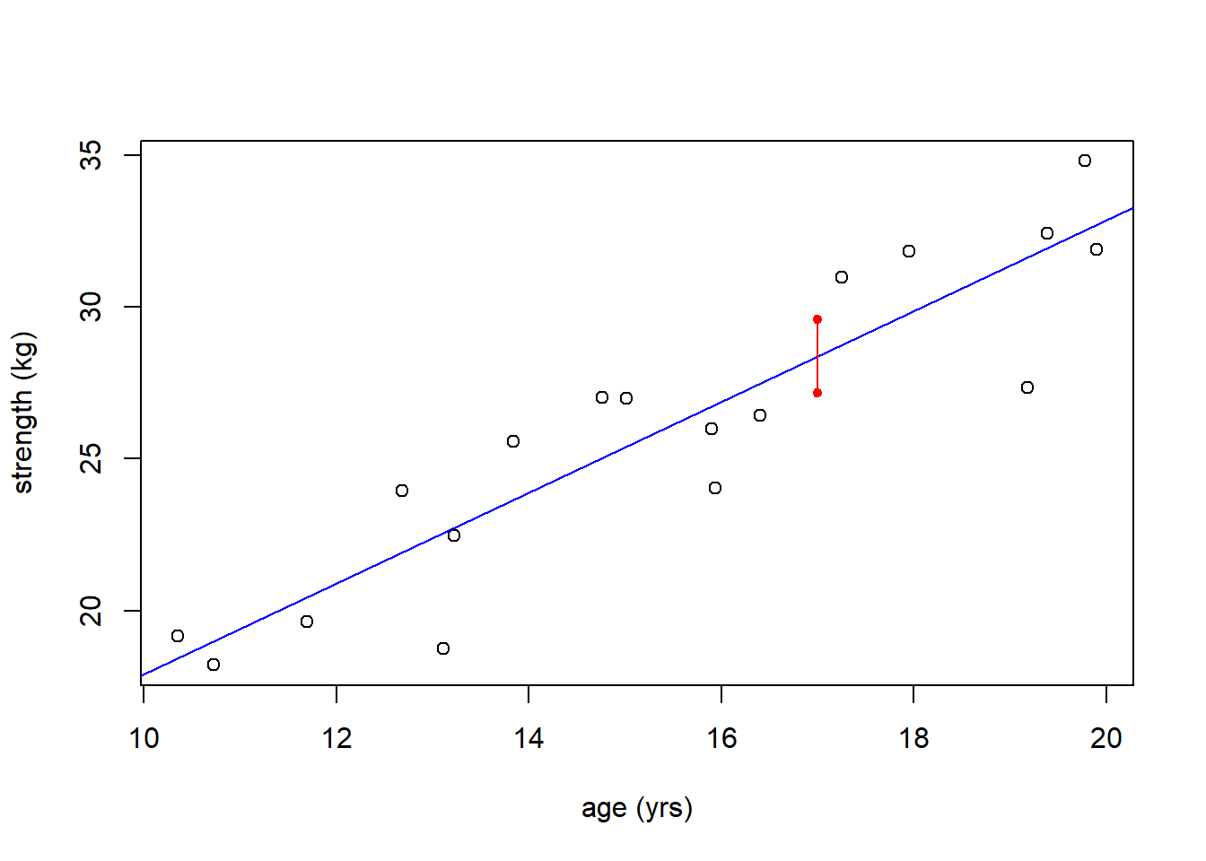

Just to confirm the fitted value if \(x^* = 17\), here are the coefficients of the fitted line:

str_age.lm$coefficients

## (Intercept)         age 
##     2.93450     1.49655

And so our “point estimate” (\(y=\beta_0+\beta_1 x\)) would then be:

2.9345+17*(1.4965)

## [1] 28.375

which matches the fitted value above.

(On a technical note, when using a fitted linear model for prediction, finding our confidence interval is not quite as easy as \(\hat\beta_1 \pm t_{df, \alpha}*SE_{\beta_1}\) because we need to take the uncertainty of both coefficients into account. The details of the math are beyond the scope of this class.)

To summarize, it’s important is that you understand what these numbers mean. Again, this interval represents the likely range of where the average \(y\) would fall for value given \(x\).

18.6.3 Calculating the Full Confidence Interval of the Prediction

Now we’re in a position to find the range of predicted average \(y\) values over the whole range of possible \(x\) values. To do this, I just need to update my newx variable to include the the wider prediction range:

newx <- data.frame(age=seq(from=10, to=20, by=0.1))

Here is the code to plot the range of predicted average results. And in fact, the dashed lines now represent the likely true range of the regression line:

plot(age, strength, xlab="age (yrs)", ylab="strength (kg)")
abline(str_age.lm, col="blue1")

conf_interval <- predict(str_age.lm, newdata=newx, interval="confidence", level=0.95)
lines(newx$age, conf_interval[,2], col="blue", lty=2)
lines(newx$age, conf_interval[,3], col="blue", lty=2)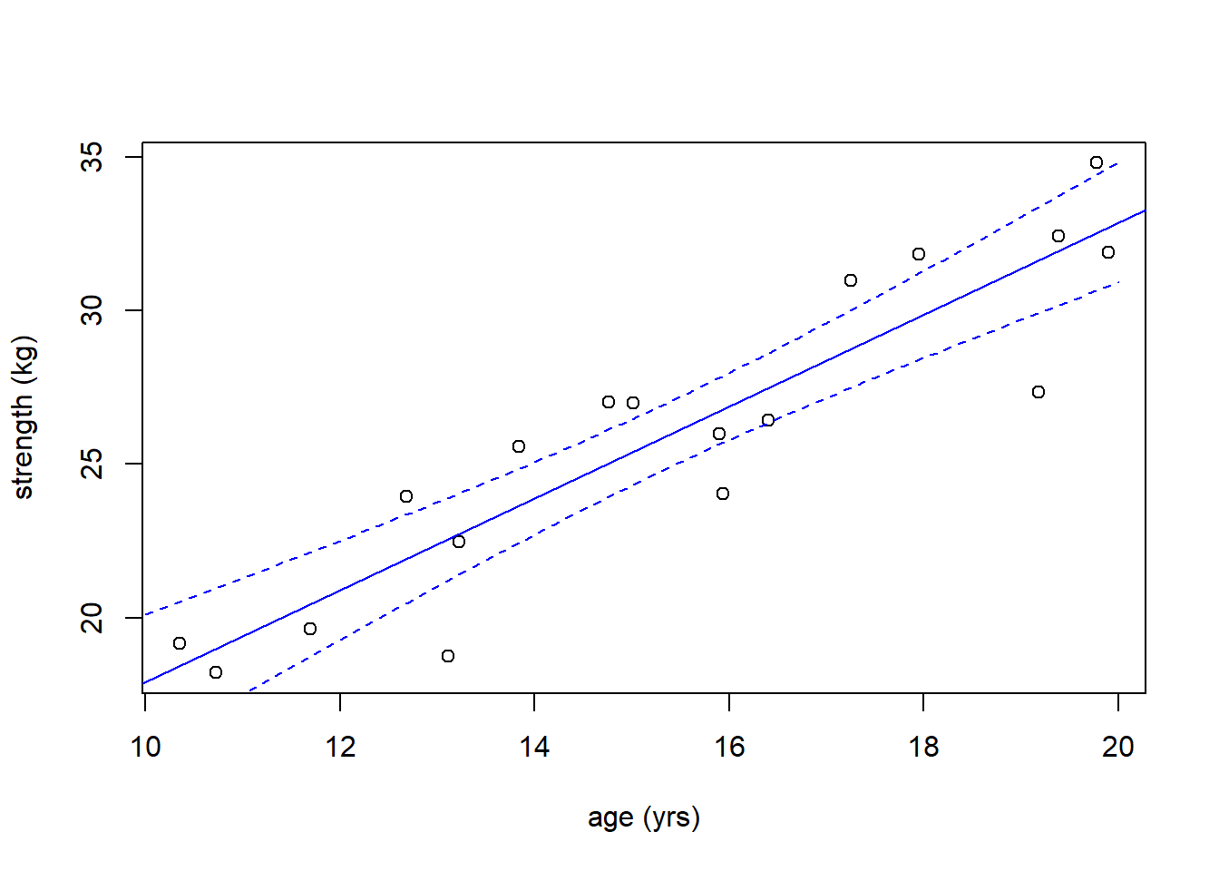

Note that a few of the points fall outside of the dashed blue curves, and that’s ok!

What we’re seeing here is the likely range of where the regression line itself might fall, not (yet) the range of any individual point. Again, what we’ve done is compute the range of an average value of \(y\) for a given value of \(x\). It’s based on both:

1. the uncertainty in the intercept parameter, which could move the line up and down, and
   
2. the uncertainty in the slope parameter, which adjusts the tilt or angle. There’s less uncertainty in the middle of the data than at the edges.

18.6.4 Predicting the Likely Range of Any Result

The second type of prediction we’ll perform concerns finding the likely range a single, individual response \(y\) might take, for a specific value of \(x\). (What’s different here is that we’re looking at an individual response instead of the average response.) We’ll call this interval a “prediction interval”.

Of note, we would only engage in prediction if we are happy with our linear model and believe that our assumptions are satisfied, particularly around the distribution of residuals.

Again for prediction, we could just calculate the point estimate: \(y^* = \beta_0 + \beta_1 x^*\), but we know that’s not that useful. Why?

Because this point estimate will (in all likelihood) be wrong. As we often saw when looking at regression lines, although the point estimate will fall exactly on the fitted line, almost none of the observed data points fell on that line. So why would we expect a new value to do so?

One other important note. Don’t make a prediction using an \(x\) value that’s outside of the range of our observed \(x\) data! Since we don’t have any data outside of our range, we aren’t sure our model is appropriate, and therefore any prediction would be suspect.

18.6.5 Uncertainty in a New Individual Prediction

As previously discussed, there is more uncertainty in a new individual prediction than there was in the distribution of the where the line lies (the average result), particularly because:

1. we need to consider uncertainty in the line itself (which was our previous effort), plus,
   
2. we also need to consider the errors, i.e. the distribution of the residuals.

Additionally, whereas when we’re thinking about the mean result, we’d use SE (a narrower range), if instead we are thinking about the range of any single value, we’d use standard deviation, which as we’ve seen throughout the year, is always larger.

The easy part here is that we simply need to change the interval type within our previous R call to "prediction". So for a single value, let \(x^*=17\) (as above):

newx <- data.frame(age = c(17))
predict(str_age.lm, newdata = newx, interval="prediction")

##        fit      lwr      upr
## 1 28.37584 23.67551 33.07618

And we see this interval {23.68, 33.08}, which represent the 95% confidence interval for any single value, is much wider than our previous estimate of where the average value might fall.

18.6.6 Visualizing Uncertainty in a New Prediction

So as we did with our confidence interval, let’s calculate and plot the prediction interval across the full range of \(x\) values:

plot(age, strength, xlab="age (yrs)", ylab="strength (kg)")
abline(str_age.lm, col="blue1")

newx <- data.frame(age=seq(from=10, to=20, by=0.1))
conf_interval <- predict(str_age.lm, newdata=newx, interval="prediction", level=0.95)
lines(newx$age, conf_interval[,2], col="blue", lty=2)
lines(newx$age, conf_interval[,3], col="blue", lty=2)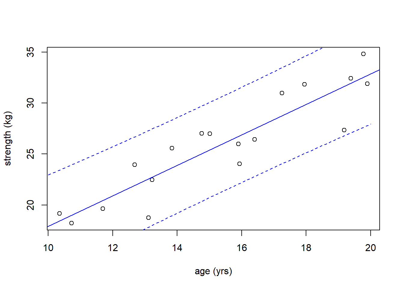

Again, in this case, these dashed lines shows the full range of expected individual values based on our model.

Of note, this new interval surrounds all of the observed data. Since our dataset only contains 18 data points, this is not unexpected at a 95% confidence level.

18.6.7 Guided Practice

Use the cars dataset to make a prediction about

1. The likely range of the average braking distance for a speed of 15 mph.
   
2. The likely range of new individual observation of braking distance for a speed of 15 mph.
   
3. Explain why the range of (b) is wider than the range of (a).

18.6.8 Possible Issues using predict()

NOTE: When using predict() be careful to make sure you match the x variable name exactly to what you used in your model call, and the easiest way to do this is to use the data= parameter in the original lm() call. So for example:

## DO THIS! 
##  Here, predict expects "speed" as the x variable name
cars.lm <- lm(dist~speed, data=cars) 
newx <- data.frame(speed=c())

## DON'T DO THIS: 
##  Here predict expects "cars$speed" as the x variable name - however this isn't easy to do.  The following doesn't quite work?!
cars.lm <- lm(cars$dist~cars$speed) 
newx <- data.frame(cars$speed=c())

So, when using data from a data frame, make sure to use the first form for the linear model with only the column names as response and predictor(s) and then pass the data frame using the data= parameter.

18.6.9 Summary and Review

Based on this section, you should now be able to:

• Discuss why a point estimate is really insufficient when making a prediction
• Explain the different types of intervals we might calculate for prediction of a new result, including:
  • Where the average result might fall, (the so-called “confidence interval of the prediction”), and
    
  • Where any individual result might fall, (the “prediction interval”)
    
• Explain why there is more uncertainty in predicting the range of any individual value compared with the range of the average value
• Describe why the average predicted value and the range of regression lines are the same
• Use the predict(..., interval="confidence") function to calculate a 95% confidence interval on where the mean value of \(y\) will fall for a given value of \(x\).
• Use the predict(..., interval="prediction") function to calculate a 95% prediction interval describing the likely range of where a single value of \(y\) might occur for a given value of \(x\).
• Explain why it is inappropriate to make a prediction using an \(x\) value that’s outside of the range of our observed \(x\) data

18.6.10 Summary of R functions

function	description
predict()	predicts an 95% (or other) confidence interval for a given linear model

 

If my.lm is a fitted linear model and newx is a dataframe containing a range (1 or more) of new \(x\) values at which to make a prediction, then to predict the range of the average (mean) response use:

predict(my.lm, newdata = newx, interval="confidence")

And to predict the range of an individual response use:

predict(my.lm, newdata = newx, interval="prediction")

18.7 Exercises

Exercise 18.1 What can you say about the following data?

x2 <- c(17.84, 14.44, 19.60, 11.02, 18.56, 10.41, 10.41, 14.76, 19.96, 13.58, 16.88, 17.23, 13.85, 12.50, 13.11, 12.01, 14.79, 17.78, 15.96, 18.88, 12.50, 13.89, 15.54, 15.95, 15.40)
y2 <- c(8.09, 6.96, 6.87, 8.24, 9.23, 10.05, 8.26, 6.58, 8.40, 8.09, 9.37, 7.28, 9.27, 8.66, 7.55, 7.43, 7.69, 6.33, 9.21, 8.40, 7.76, 8.86, 6.96, 8.48, 9.10)

 

Exercise 18.2 Skim the following website to learn about ground level ozone: https://www.epa.gov/ground-level-ozone-pollution/ground-level-ozone-basics

Using the airquality data (which is built in to R), create two different scatter plots, using the plot() function. The first one should show Ozone against Solar.R and the second should show Ozone against Temp. Use appropriate x- and y-axis label names. For each case, if you can, discuss why one variable should be the predictor and the other should be the response variable?

In words, describe both plots, include any relationship you see. In particular, attempt to answer the questions in section 17.3.2.

 

Exercise 18.3 Again, using the airquality data, answer the following questions:

1. Calculate the correlation between Ozone and Solar.R
   
2. Calculate the correlation between Ozone and Temp
   
3. Explain what the results of parts (a) and (b) and the previous problem suggest about whether Solar.R or Temp may have a stronger influence on Ozone. Be specific and quantitative in your answer.
   

 

Exercise 18.4 The following data shows Women’s earnings as a percentage of Men’s for full time wage and salary workers 1979 to 2018, taken from the US Bureau of Labor Statistics (https://www.bls.gov/cps/earnings.htm).

1. Create a vector that contains all years from 1979 to 2018 and then use this to create a scatter plot of earnings vs. time. (Hint: use seq()) Explain why you choose your predictor and response variables.
   
2. Use a few sentences to describe the relationship you see in the scatter plot. In particular, attempt to answer the questions in section 17.3.2.
   
3. Calculate the correlation between year and the women’s earnings data. What do these values suggest?
   

ws <- c(62.3, 64.2, 64.4, 65.7, 66.5, 67.6, 68.1, 69.5, 69.8, 70.2, 70.1, 71.9, 74.2, 75.8, 77.1, 76.4, 75.5, 75.0, 74.4, 76.3, 76.5, 76.9, 76.4, 77.9, 79.4, 80.4, 81.0, 80.8, 80.2, 79.9, 80.2, 81.2, 82.2, 80.9, 82.1, 82.5, 81.1, 81.9, 81.8, 81.1)

 

Exercise 18.5 Pick two of the variables below and attempt to weave an explanation of why they might be correlated with each other. Make sure to describe whether you would expect a positive or negative relationship, as well as whether there is a causal relationship or potentially some other common covariate.

1. Number of wins for the Sounders
2. Restaurant sales in Seattle
3. Revenues of tech companies with offices in the Seattle greater area
4. Gas prices in the PNW
5. Transportation related carbon emissions in Washington State
6. Minimum hourly wage for restaurant workers in Seattle
7. Percent of students in the Puget Sound region attending private school
8. Number of days per month with temperature above 70 degrees F

 

2. What are some examples of data that are correlated and causally linked?
   
3. What are some examples of data that are correlated and probably not causally linked, but possibly have a common covariate?
   

 

Exercise 18.6 Using the faithful data (which is built in to R):

1. Create a well formatted scatter plot showing the relationship between waiting time and eruption length. Which is the best predictor variable and which is the best response variable?
   
2. Fit a linear model and overlay the fitted result on the plot. Comment on what you think about the fit.
   
3. Extract the parameters of the model. Interpret what the value of the slope and intercept represent.
   
4. Based on the coefficients, calculate the fitted values using vector math. Compare your results to the $fitted.values result.
   
5. Calculate the residuals using vector math. Compare your results to the $residuals result. What do your residuals sum to?
   
6. Plot the residuals as a function of your x variable. Comment on what you observe? Does the assumption of a random (Normal) distribution seem appropriate?
   

 

Exercise 18.7 Using the faithful data, evaluate if waiting time is a significant predictor of eruption length:

1. Fit a linear model (you may have already done this in the previous problem).
   
2. What are the coefficient estimate and standard error for the slope parameter? Using those, calculate the test statistic, and then, based on the appropriate degrees of freedom, determine the p-value. Confirm your results match the summary() output.
3. What do you conclude about the \(H_0: \beta_1=0\)?
   
4. What is a 95% confidence interval around \(\beta_1\)? How does that result compare to your answer for part (c)? Hint: \(\hat \beta_1 \pm t_{df, \alpha}*SE_{\beta_1}\)
5. What is the \(R^2\) value and what does it suggest about our model? Then, calculate the correlation (using cor() and prove to yourself that \(R^2\) is in fact the square of the correlation).
   

 

Exercise 18.8 Explain in a few sentences why there is uncertainty in our coefficient estimates.

 

Exercise 18.9 Explain in a few sentences why we typically care more about whether \(\beta_1=0\) than if \(\beta_0=0\).

 

Exercise 18.10 The following data shows Women’s earnings as a percentage of Men’s for full time wage and salary workers 1979 to 2018, taken from the US Bureau of Labor Statistics (https://www.bls.gov/cps/earnings.htm).

1. Create a vector that contains all years from 1979 to 2018 and then use this to create a scatter plot of earnings vs. time. (Hint: use seq()) You may have already done this in a previous exercise.
2. Create a linear model using year as the predictor and women’s pay as the response. Add the fitted line to the plot and comment on whether you think it’s a good fit. What is the \(R^2\) value? How does your interpretation of the \(R^2\) value correspond to what the plot shows?
   
3. Plot the residuals as a function of year. Does they seem to be randomly distributed or does there seem to be any type of trend?
   
4. Based on the summary table, what do you conclude about \(\beta_1\)?
   
5. Based on parts a..d, comment about whether/if we can find significant predictors even when our model is suspect.
   

ws <- c(62.3, 64.2, 64.4, 65.7, 66.5, 67.6, 68.1, 69.5, 69.8, 70.2, 70.1, 71.9, 74.2, 75.8, 77.1, 76.4, 75.5, 75.0, 74.4, 76.3, 76.5, 76.9, 76.4, 77.9, 79.4, 80.4, 81.0, 80.8, 80.2, 79.9, 80.2, 81.2, 82.2, 80.9, 82.1, 82.5, 81.1, 81.9, 81.8, 81.1)

 

Exercise 18.11 Use the above code in Section 17.5.5 to generate different sampled \(y\) values, based on the idea that our model is right and that you can randomly assign residuals to different fitted values.

1. By hand, run this code a number of times. What do you observe about how often our initial parameter estimates are correct?
   
2. Write some code that allows you to extract the parameter value for \(\beta_1\) for each simulation. Note my.lm$coef[2] or similar should work.
   
3. Run this process 40 times and then calculate the mean and standard deviation on \(\beta_1\). How do these compare to the coefficient table?
   

 

Exercise 18.12 In this exercise, you will use the following code to generate random points and then fit a linear model to those points. In this case, you will already know the coefficients of the line (because we are simulating them), and you are testing to see how well our model fitting process works.

1. Run the following code as is a few times. Each time, a new dataset is generated because of the rnorm() call, which generates and assigns random residuals to each point. How much do the plot or summary results change? How close are the fitted values to the true values?
2. What about the summary output can you use to evaluate if our estimates of beta0 and beta1 are approximately correct?
   
3. Increase the value epsilon and then simulate the data and fit the model. Now how close are the fitted values to the true values? Does our ability to correctly estimate a parameter get better or worse as \(\epsilon\) increases?
   
4. Now increase \(n\) to experiment with different sample sizes. Does our ability to correctly estimate a parameter get better or worse as \(n\) increases?
   

beta0 <- 4.2
beta1 <- 1.8
epsilon <- 1.8
n <- 10 

x3 <- runif(n, 0, 10)
y3 <- beta0+ beta1*x3 + rnorm(n, 0, epsilon)

plot(x3, y3)
my.lm3 <- lm(y3~x3)
abline(my.lm3)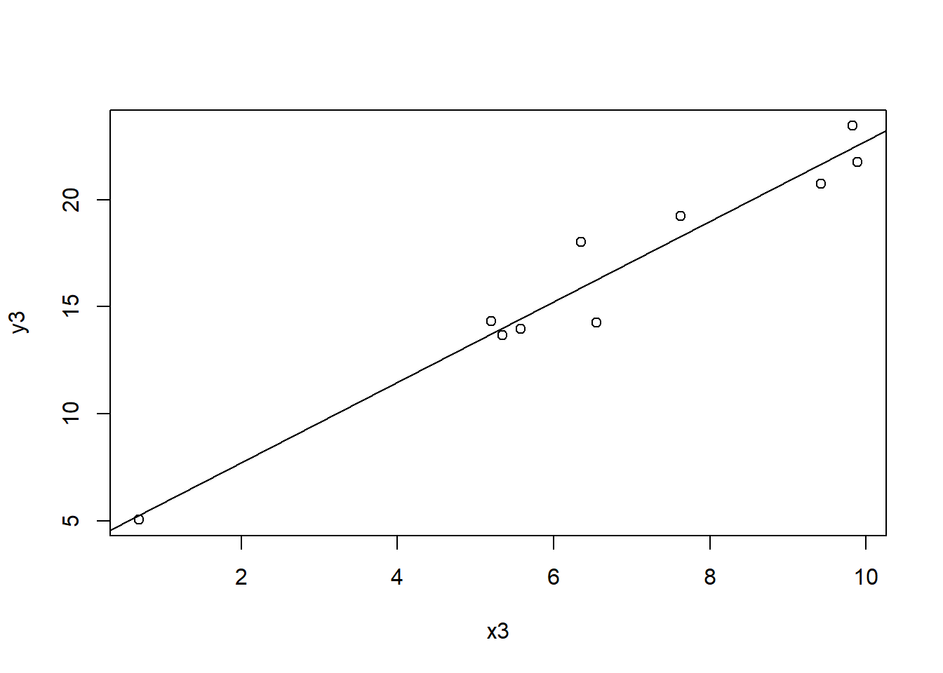

summary(my.lm3)

## 
## Call:
## lm(formula = y3 ~ x3)
## 
## Residuals:
##     Min      1Q  Median      3Q     Max 
## -2.0127 -0.7128 -0.2663  0.8706  2.1504 
## 
## Coefficients:
##             Estimate Std. Error t value Pr(>|t|)    
## (Intercept)   3.9625     1.0849   3.652  0.00647 ** 
## x3            1.8784     0.1517  12.386 1.68e-06 ***
## ---
## Signif. codes:  0 '***' 0.001 '**' 0.01 '*' 0.05 '.' 0.1 ' ' 1
## 
## Residual standard error: 1.267 on 8 degrees of freedom
## Multiple R-squared:  0.9504, Adjusted R-squared:  0.9442 
## F-statistic: 153.4 on 1 and 8 DF,  p-value: 1.684e-06

 

Exercise 18.13 Using the faithful data (which is built in to R):

1. What is a 95% confidence interval on the slope parameter.
   
2. What does this range tell you about whether you should reject \(H_0\)?

 

Exercise 18.14 Using the following data for \(x\) and \(y\),

1. Create a plot that shows the original data, and the best fitting line.
2. Is \(x\) a statistically significant predictor of \(y\)?
   
3. How much of the variation in \(y\) is explained by our model?
   
4. What would you predict as a point estimate and a likely range for a new value of \(y\) if \(x^* =16.5\)?
   
5. What would you predict as a point estimate and a likely range for the average value of \(y\) if \(x^* =16.5\)?
   
6. Why are your answers to (d) and (e) different? Which interval is wider?

x <- c(19.39, 10.72, 10.35, 19.78, 15.94, 17.95, 15.90, 19.90, 15.01, 13.22, 11.69, 16.40, 13.84, 14.76, 12.68)
y <- c(32.42, 18.21, 19.16, 34.80, 24.04, 31.83, 25.99, 31.89, 27.00, 22.47, 19.63, 26.44, 25.56, 27.03, 23.93)

 

Exercise 18.15 Again using the above data for \(x\) and \(y\), create a plot that shows the original data, the best fitting line, and the confidence interval of the prediction, i.e. the likely range of mean values of \(y\) given all \(x\) in the range from 10 to 20.

Create 95% confidence intervals around both coefficients: \(\beta_0\) and \(\beta_1\). How do these confidence intervals relate to our null hypothesis?

 

Exercise 18.16 In a few sentences, explain why just using a point estimate for prediction might have limited usefulness.

 

Exercise 18.17 In a few sentences, discuss why the uncertainty and therefore the computed interval width of a new single prediction of \(y\) is much larger than range of the average value of \(y\) given \(x\).

 

Exercise 18.18 In the lecture notes, graphs were presented including those that computed both the 95% confidence and prediction intervals. What do you expect would happen to these interval widths if we computed a 99% confidence interval? Try it using the cars data and confirm your guess.