Chapter 7 Expected Value and Variance of Discrete Random Variables
7.1 Overview
We previously talked about discrete variables, basically those where the outcomes can only be a discrete set of values. Examples include:
- the role of a die (outcomes: 1, 2, 3, 4, 5, or 6)
- the number of heads in 3 coin flips (outcomes: 0, 1, 2, or 3)
- the color of skittle drawn (outcomes: P, R, O, Y, G, or B)
- whether you win, lose or tie in a game of chance
Here, we’ll discuss and quantify the mean and variance of those types of random variables, and introduce the concept of expected value.
7.1.1 Shall we play a game?
Imagine the following game. It costs $15 up front to play. You roll 2 dice. If the sum is 2, 3, or 12 you win $100. If the sum is 7 or 11 you get your money ($15) back. For any other sum (4, 5, 6, 8, 9, or 10), you win nothing and lose your $15. Should you play?
- take some dice and play with a partner. Record your results.
- use the
sample(1:6, 1)command in R to simulate a die roll and record your results.
| game | roll | $ win/loss | running total |
|---|---|---|---|
| 1 | |||
| 2 | |||
| 3 |
What do you think of this game? Would you play? What information are you using to make that decision?
As we’ll see in this chapter, this approach of understanding and quantifying uncertainty and risk has applications beyond simple games.
7.1.2 Learning Objectives
By the end of this chapter you should be able to:
- Explain what a discrete random variable is and give examples
- Define what expected value means, namely the long term expected average, or the probability weighted average
- Calculate both the expected value and expected variance (and standard deviation!) of a discrete random variable, both by hand and using vector math in R
- Discuss the relationship between z-scores and the chance of losing money for well behaved data
- Explain how we can use the expected value result in decision making
- Define risk averse, risk neutral and risk prone
- Describe the relationship between the size of the simulation and its precision
7.2 Expected Value Analysis
If you roll a single fair, six-sided die, what is the expected result? It’s probably a bit hard for you to choose one answer, right, because each outcome has the same probability. So what if I asked about the sum of two die, is that easier? In that case, rolling a 7 has the highest probability, so maybe that’s what’s “expected”?
In fact, the term “expected” has a specific meaning in this context.
Generally, when I say the expected result, what I mean is the average result if we rolled a die many, many times. And we will extend this shortly when our outcomes are more than just the roll of a die.
One other important note is that under this definition, the expected result doesn’t describe the variation in results that exists. We’ll come that in a bit.
How might we calculate the expected value, given this definition? Well, what does it depend on? Certainly both:
- the different outcomes, and
- the probabilities of those outcomes
Formally, if \(X\) is a random variable that describes the outcome of a single die roll (again, a random variable means we don’t know the value until after the event happens), then the Expected Value of \(X\), which we’ll write as \(E[X]\) is:
\[E[X] = \sum_{i=1}^n X_i P_i\]
Where:
- \(\sum\) means sum
- \(i\) is an index
- \(n\) is the total number of different outcomes
- \(X_i\) is the value of outcome \(i\), and
- \(P_i\) is the probability of observing outcome \(i\)
The right hand side of this equation says that we are summing the product of each outcome times its probability.
7.2.1 Rolling One Die
Let’s apply this equation to the roll of one die. What is the expected value of that roll?
\[\begin{eqnarray*} E[X] & = & \sum_{i=1}^n X_i P_i \\ & = & 1* \frac{1}{6} + 2* \frac{1}{6} + 3* \frac{1}{6} + 4* \frac{1}{6} + 5* \frac{1}{6} + 6* \frac{1}{6} = \frac{21}{6} = 3.5 \end{eqnarray*}\]
The expected value is the long term average (mean) result.
Can we ever role a 3.5? In fact, no. Also, it’s not necessarily the mode, the most frequent occurrence.
7.2.2 Guided Practice
- what is the expected value of a four-sided die?
- what is the expected value of the sum of rolling two six-sided die? Give me your guess and then solve using the expected value calculation. Hint: you’ll first have to figure out what the possible outcomes and the associated \(P_i\) are.
- If we play a game where you lose $1 for flipping a H and win $1 for flipping T, assuming a fair coin, what is the expected value?
7.2.3 Simulation in R and the Law of Large Numbers
Let’s use R to simulate a large number of rolls and see what the average result is:
## The number of rolls
nrolls <- 10000

## Create a numeric vector to store the results
rslt <- vector("numeric", nrolls)

## Use a for loop to roll the die nrolls times and store the result
for (i in 1:nrolls) {
  rslt[i] <- sample(1:6, 1, replace=T)
}

## Calculate the average of all my rolls
mean(rslt)
## [1] 3.4978The Law of Large Numbers says that if you sample something many, many times, the sample tends toward the true value.
From Wolfram, “the ‘law of large numbers’ is one of several theorems expressing the idea that as the number of trials of a random process increases, the percentage difference between the expected and actual values goes to zero.”
7.2.4 Guided Practice
- Use simulation in R to show that \(E[X]\) for the sum of 2 dice is the same as the long term average. Hint, remember you can use
sample()to generate random data.
7.3 Shall We Play A Game?
We can use the expected value analysis for some more interesting questions and lots of applications where we can estimate both a set of outcomes and their associated probabilities.
Imagine the following game (different/simpler than the one in our introduction). Here are the rules:
- Roll one die.
- If you roll a 1 or 2 you win $10.
- If you roll a 3, it is a push (meaning no win or loss)
- If you roll a 4, 5, or 6, you lose $5.
Would you play? How would you decide?
In fact, your answer probably depends a bit on your risk tolerance, which we’ll get into in a bit. For now, let us start by calculating the expected value for this game.
Remember, \[E[X] = \sum_{i=1}^n X_i P_i\]
First, what are the \(X_i\) here? And, what are the \(P_i\)? And what is \(i\) and \(n\)?
| i | 1 | 2 | 3 | 4 | 5 | 6 |
|---|---|---|---|---|---|---|
| \(X_i\) | $10 | $10 | $0 | -$5 | -$5 | -$5 |
| \(P(X_i)\) | 1/6 | 1/6 | 1/6 | 1/6 | 1/6 | 1/6 |
Note that our outcomes here are not the die results, but the amount of money we win or lose in each case.
And so based on this we multiply the probabilities and winnings for each outcome (in each column) and then add those products together to find \(E[X] = 10 * \frac{1}{6} + 10 * \frac{1}{6} + 0* \frac{1}{6} - 5*\frac{1}{6} - 5*\frac{1}{6} - 5*\frac{1}{6} = \frac{5}{6}\)
What does this value, \(E[X]= \frac{5}{6}\) represent? It’s the expected long term average if we were to play this game many, many times. On average for this game we’d expect to win \(\frac{5}{6}\) dollars per turn. And remember, based on the rules we can’t actually win that amount on any single turn.
Now, what does this result tell us about whether we should play this game? Since the expected value is greater than 0, that means on average we would come out positive. Assuming we’re willing to take the risk of losing money along the way, we should be willing to play, because over the long term, we’ll come out ahead.
7.3.1 Guided Practice
- For the above game, if we only win $7.50 on a 1 or a 2, what is the new expected value? Does that change your decision about whether to play?
7.4 Expected Variance
So the expected value gives us a point estimate, which is the long term average, and we know that a random variable also has variation in any given turn, roll, draw, or trial. So ideally, to answer the question of “would we play”, we want to quantify this variability. How much spread is there in the average result?
For a discrete random variable we can do this explicitly and calculate the variance based again on \(X_i\) and \(P_i\).
Formally we can write:
\[Var[X] = E[X^2] - (E[X])^2\]
I won’t derive this here, but note that it’s at least similar to the variance calculation we did previously.
We’ll approach this in two steps, by first calculating \(E[X]\) and \(E[X^2]\) separately, and then combining them to find \(Var[X]\).
7.4.1 Variance of a Single Die
As our first example, let’s go back to the roll of a single six-sided die, not the game (yet).
For this, we already found \(E[X] =3.5\) above. So we can calculate \((E[X])^2 = 3.5^2 = 12.25\). So our first step in determining variance is to find \(E[X]\) and then square it.
How would we find \(E[X^2]\)?
To do this, we need to know the outcomes and associated probabilities of \(X^2\), where the probabilities of \(X^2\) are simply the probabilities of \(X\). So given:
\[E[X^2] = \sum_{i=1}^n X_i^2 P_i\]
For our single die roll we can then write:
\[E[X^2] = \sum_{i=1}^n X_i^2 P_i = 1^2 * \frac{1}{6} + 2^2 * \frac{1}{6} + 3^2 * \frac{1}{6} + 4^2 * \frac{1}{6} + 5^2 * \frac{1}{6} + 6^2*\frac{1}{6} = \frac{91}{6} = 15 \frac{1}{6}\]
As before, we multiply the observed value of \(X_i^2\) times the probability of each \(X_i\) first (again the probabilities don’t change), and then sum all the results.
For our final step, we put these results together to find \[Var[X] = E[X^2] - (E[X])^2 = 15\frac{1}{6}-12\frac{1}{4} = 2\frac{11}{12}\]
What does this value represent? This is the variance of one roll of a die. As previously discussed, it’s probably more useful to look at the standard deviation, which is \(\sqrt{2\frac{11}{12}} = 1.708\). Remember that standard deviation is in the same units as our data.
We’ll discuss how to interpret this value shortly, but given we now know the mean and standard deviation, you might begin to think about our rules of thumb here.
7.4.2 The Variance of our Game
Let’s repeat the variance calculation for our single die game from above. We found that the expected value of that game was \(\frac{5}{6}\). What about the expected variance?
Here is our table for outcomes and probabilities and note I have now also added a row for the \(X_i^2\):
| i | 1 | 2 | 3 | 4 | 5 | 6 |
|---|---|---|---|---|---|---|
| \(X_i\) | $10 | $10 | $0 | -$5 | -$5 | -$5 |
| \(P(X_i)\) | 1/6 | 1/6 | 1/6 | 1/6 | 1/6 | 1/6 |
| \(x_i^2\) | 100 | 100 | 0 | 25 | 25 | 25 |
Here I’m using the amount we win or lose as our outcome and our probabilities of each outcome are unchanged.
Based on this we find the \[E[X^2] = \sum_{i=1}^n X_i^2 P_i = 100 * \frac{1}{6} + 100 * \frac{1}{6} + 0 * \frac{1}{6} + 25 * \frac{1}{6} + 25 * \frac{1}{6} + 25 * \frac{1}{6} = \frac{275}{6} = 45 \frac{5}{6}\]
Then to find \(Var[X]\), we compute
\[Var[X] = E[X^2] - (E[X])^2 = 45 \frac{5}{6} - \left(\frac{5}{6}\right)^2 = 45 \frac{5}{36}\]
which gives a standard deviation (the square root) of approx $6.72. Did you forget about the units? Standard deviation has the same units as the original data, so the units here are $.
7.4.3 Interpreting the Var[X] for One Roll
How should we interpret the variance of standard deviation of the expected value? You might think about our rules of thumb and intervals. For example, the expected value is positive ($0.833), AND we also see that losing money is well within one standard deviation ($6.72) of the mean.
But honestly, this is over complicating things. What is the probability of losing money on any (one) turn?
Here is a plot showing the distribution of winnings with the expected value shown in dark green.
As we’ve seen, although the expected value is positive, losing money is still a very likely outcome of any single turn! In fact, the probability of losing money on any given turn is 50%.
x <- c(-10, -5, 0, 5, 10)
p <- c(0, 3/6, 1/6, 0, 2/6)
barplot(p, names.arg=x, ylim=c(0, 0.75), xlab="Winnings", ylab="Probability")
abline(v=2.5+5/6, lty=2, col="dark green")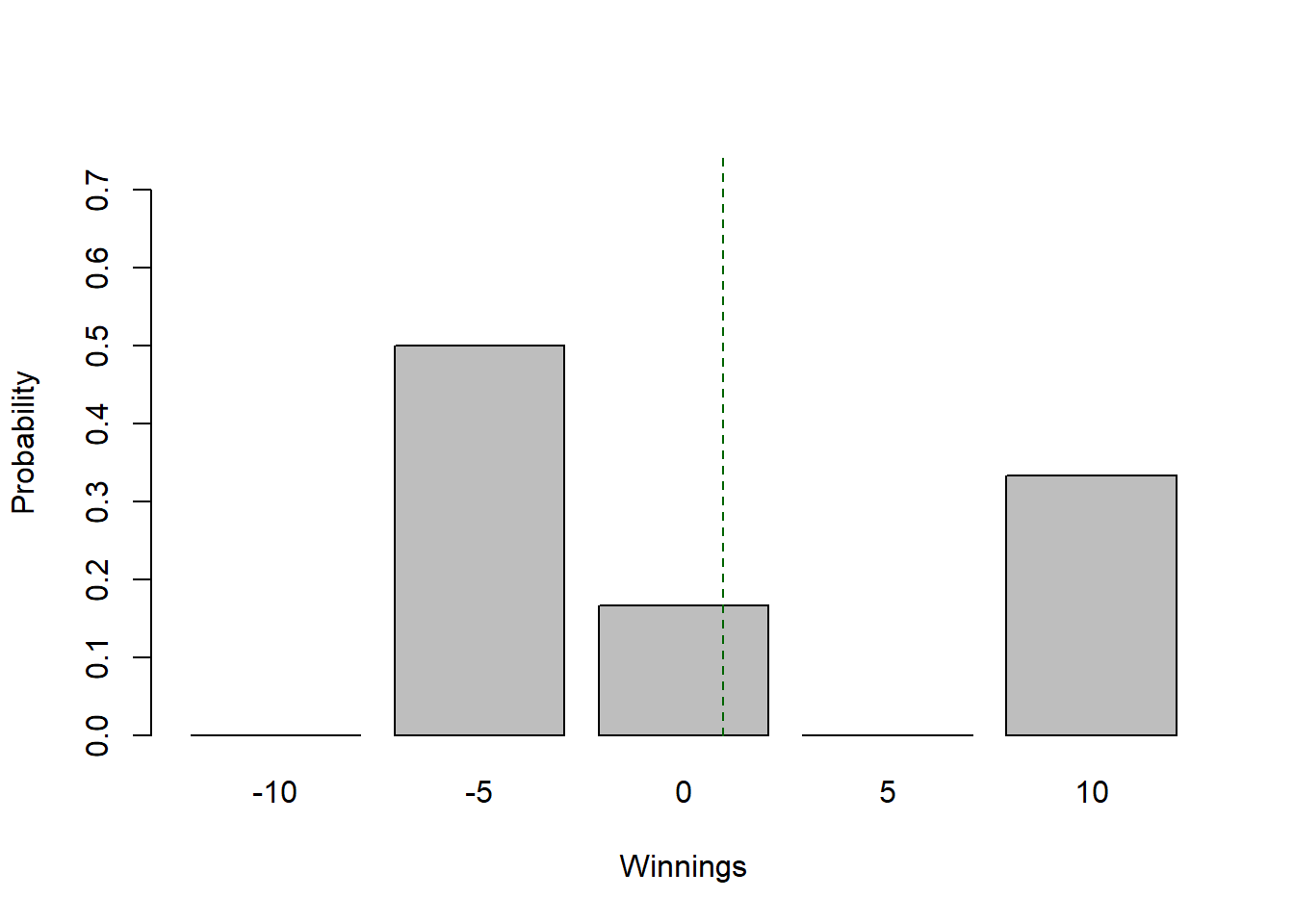
So, what does this mean? For now, simply recognize that we can calculate the standard deviation, but know that it will have more meaning when we examine the results of more turns.
7.4.4 Calculating E[X] and Var[X] in R
Above we did all these calculations for \(E[X]\) and \(Var[X]\) by hand which can be a little tedious and is error prone. In fact, R is pretty good at doing these types of calculations, particularly using the vector math approach we learned previously.
Here I’ll demonstrate the using R to calculate the expected value for our single die game.
To do so, first we set up a vector with the probabilities, where rep() stands for repeat:
## [1] 0.1666667 0.1666667 0.1666667 0.1666667 0.1666667 0.1666667Or, alternatively it can be as simple as:
Then create a vector with the outcomes:
## [1] 10 10 0 -5 -5 -5The elements in the probability vector must align with those in the outcome vector. So, the first element in the probability vector must correspond to the first element in the outcome vector, and so on.
Next, in R, we can use vector math to multiply these as:
## [1] 1.6666667 1.6666667 0.0000000 -0.8333333 -0.8333333 -0.8333333This does multiplication on an element by element basis, so the first element of the result is the first element of p times the first element of x, and so forth.
We can easily sum this vector, resulting in the \(\sum X_i P_i\) - the expected value, which matches our above calculation.
## [1] 0.8333333Let’s now use this same approach calculate the variance. We can square the x vector on an element by element basis using:
## [1] 100 100 0 25 25 25and so similar to above we calculate the expected value of \(E[X^2]\) as:
## [1] 45.83333Then, we can combine these to calculate the variance as:
## [1] 45.13889which also matches our results from above.
Finally, to find the standard deviation, we can use:
## [1] 6.718548And be careful here that the outer parenthesis surround the entire calculation.
7.4.5 Guided Practice
- What is the variance of the sum of 2 dice? Do this by hand and using vector math in R to confirm your results.
7.4.6 Simulating our Results
See the “expected-value-simulation.R” script (modified 11/09/20 to match the review problem.)
- Download the script from Canvas and press the Run button to make sure it loads. You may need to download the
svDialogspackage. - Run the
play.once(T)function by typing this into the console. What do you observe? - As a class, let’s do the simulation together. Press the Source button and then report out your results. Let’s run the game with 10, 100, 1000, 10000, etc. and put results into Excel. What do you observe about the results as
ngamesgets bigger?
Now, how much would you be willing to pay to play this game? How would we change this to make it so that it costs that much to play each time? How would that change our expected results?
7.4.7 Guided Practice
- It costs you $15 to play. You get to roll 2 dice. If the sum is 2, 3 or 12, you win $100. If the sum is 7 or 11, you get your money back. If any other sum (4,5, 6, 8, 9, or 10) you win nothing and lose your $15. Would you play? And how would you decide?
You could use your dice and play with this for a little while. Maybe do 20 rolls, keeping track of your wins and losses.
| turn | roll | outcome |
|---|---|---|
| 1 | ||
| 2 | ||
| … |
- Calculate the \(E[X]\) and \(Var[X]\) for this game. (Hint: create a table that shows the outcomes in $ and associated probabilities.)
- Would you play? Why or why not?
- Now, modify the R script for this game and run it a large number of times. Do your hand calculations and simulated results match?
7.4.8 Summary of Computing E[X] in R
For the two dice game we would use:
# load the probability vector and ensure it equals 1
prob <- c(1/9, 2/9, 2/3)
paste("The sum of the probabilities is:", round(sum(prob), 3))
## [1] "The sum of the probabilities is: 1"# load the outcome vector
outcome <- c(85, 0, -15)
# the expected value is the sum of the element-wise outcomes * probabilities
exp.val <- sum(outcome * prob)
paste("The expected value is:", round(exp.val, 3))## [1] "The expected value is: -0.556"# the expected variance is E[X^2] - (E[X])^2
exp.vari <- sum(outcome^2 * prob) - (sum(outcome * prob))^2
paste("The variance is:", round(exp.vari, 3))## [1] "The variance is: 952.469"# the expected standard deviation is \sqrt(E[X^2] - (E[X])^2)
paste("The standard deviation is:", round(sqrt(exp.vari), 3))## [1] "The standard deviation is: 30.862"You’ll note I’ve added a few new function here, paste() and round(). The paste() function is useful to print out a combination of text and calculations. The output will show after the chunk is run. The round() function simply rounds a calculated value to the specified number of decimal places.
7.4.9 E[X] and Var[X] of Many Turns
Here I’m going to introduce a concept that we will come back to in a later chapter.
In our game above we found \(E[X] = 0.833\) and \(Var[X] = 45.139\) for one turn. What happens if we play the game \(n=100\) times? In particular, what are the mean and variance of the cumulative results?
If we play the game \(n=100\) times, then the expected value is \[n*E[X]= 100*(0.833) = 83.33\] This result is probably fairly intuitive. The results of individual turns simply add together.
What about the spread (standard deviation)? The standard deviation of the cumulative results from \(n\) games is \[\sqrt{n}*SD[X]\] and the distribution is "well-behaved". (Why? We will discuss and derive the details of this equation and why it comes about next Trimester. For now we will focus on what it means and how to use it.)
Above we found \(Var[X] = 45.139\), which means the standard deviation after \(n=100\) games would be \(\sqrt{45.139*100} = 67.19\). Let’s attempt to visualize what that means.
You should remember from an early chapter that 95% of our distribution will lie in the interval between the mean plus or minus twice the standard deviation.
Here is a histogram of the expected cumulative result from playing \(n=100\) games, with the expected value indicated in dark green, and the likely 95% interval highlighted in red.
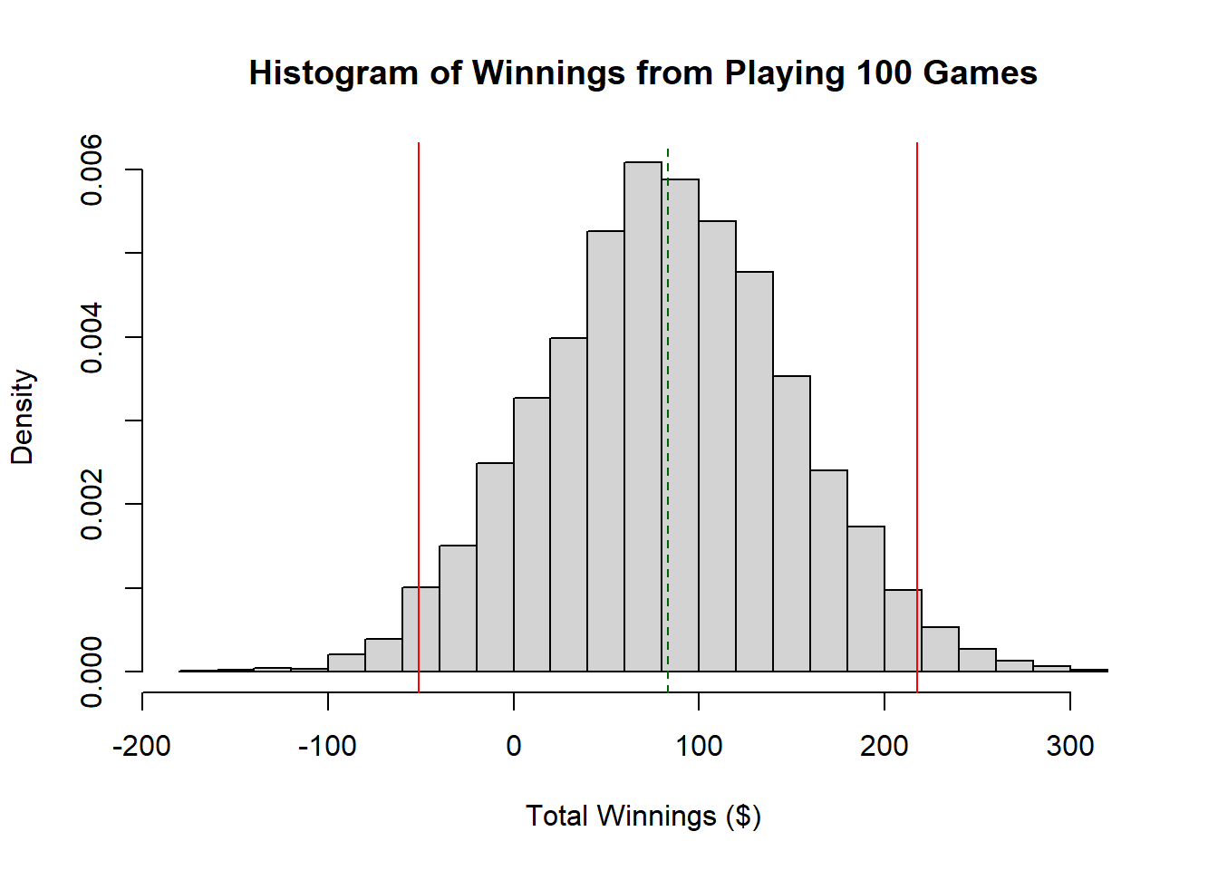
How does this help us decide if we would play?
7.4.10 Z-scores of 0
Remember our z-scores? How many standard deviations away from zero is the expected value?
For 100 turns we can find this as \(\frac{x-\mu}{\sigma} = \frac{0-83.33}{67.19} = -1.24\). This means losing money (i.e. a result less than 0) is -1.24 standard deviations away from 0.
NOTE: the order of \(x=0\) and \(\mu=E[X]\) is critical here!
## [1] 0.1074877We can see from the above histogram that there is a sizeable portion of the distribution below zero, meaning there is a good chance of losing money.
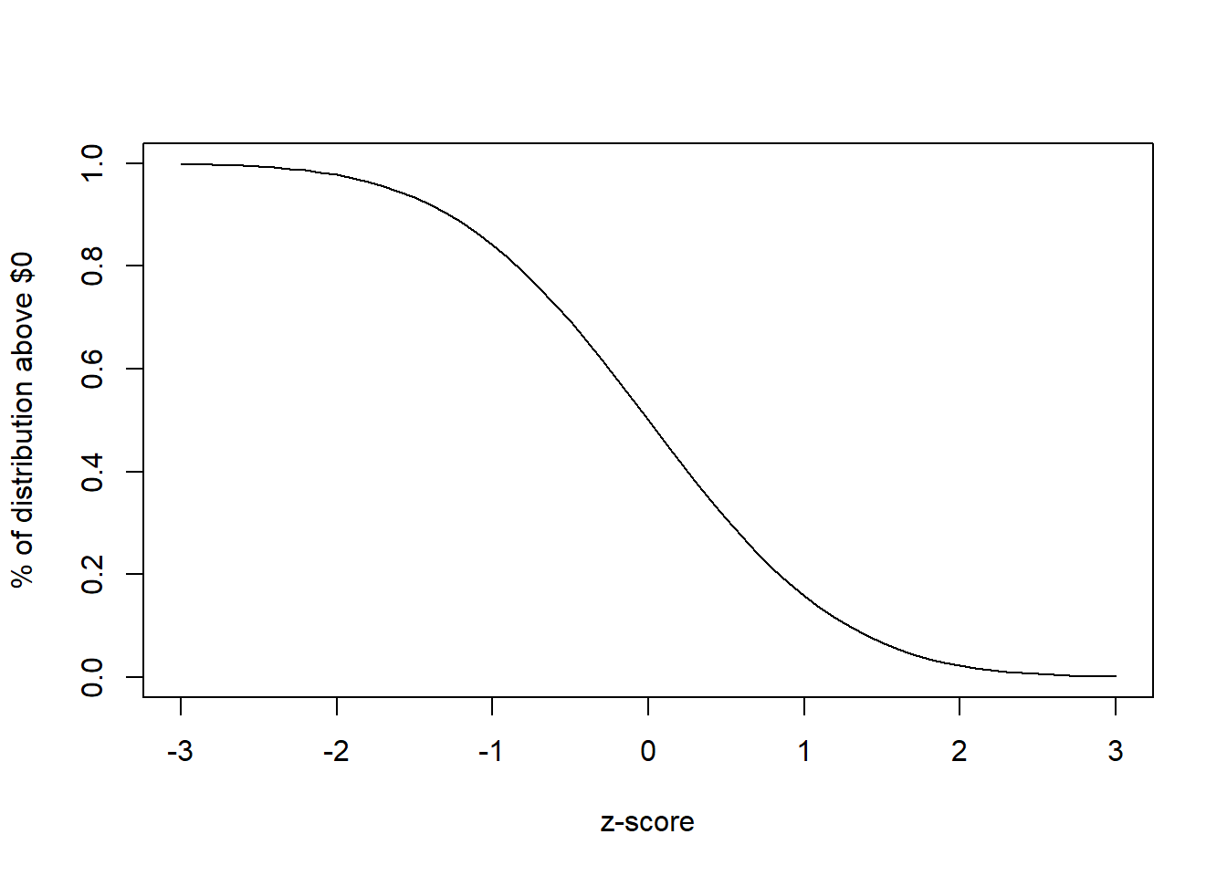
In a later chapter we’ll learn how to quantify this “good chance” more precisely. In fact, based on the assumption of Normality, 10.7% of this distribution is below zero this and so 89.3% is above zero. That means (if the assumptions of Normality held), that 89% of the time, we would expect our winnings will be above 0. We don’t quite have the tools do to this calculation yet, so the following table gives a rough approximation of the relationship between z-scores and the probability of losing money for well behaved data:
| z-score of 0 | % of distribution above 0 |
|---|---|
| -3 | 99.8% |
| -2.5 | 99.4% |
| -2 | 97.7% |
| -1.5 | 93.3% |
| -1 | 84.1% |
| -0.5 | 69.1 |
| 0 | 50% |
| 0.5 | 30.9% |
| 1 | 15.9% |
| 1.5 | 6.7% |
| 2 | 2.3% |
| 2.5 | 0.6% |
| 3 | 0.2% |
For example, a z-score of -2.5 means that 0 is 2.5 standard deviations below the expected result, so there’s little chance of losing money. Alternatively, a z-score of +1.5 means that 0 is 1.5 standard deviations above the expected value, so there’s roughly a 6.7% chance of coming out positive.
And for z-scores in between listed values, you can simply interpolate.
The key takeaway for now is that we can use the standard deviation (and mean) within a z-score analysis to evaluate how likely it is for us to lose money. The more negative the z-score, the better our results.
And here is a plot of the same results:
7.4.11 Guided Practice
For a game with an expected value of \(\mu=0.67\) and expected standard deviation of \(\sigma=1.2\), what is the z-score of \(0\)? What is the approximate probability of negative winnings?
For a game with an expected value of \(\mu=-0.25\) and expected standard deviation of \(\sigma=.25\), what is the z-score of \(0\)? What is the approximate probability of negative winnings?
7.5 Using Expected Value in Decision Making
The approach we’ve used above to decide whether we’ll play has assumed that we are risk neutral and that we have enough money to cover our losses while the Law of Large Numbers kicks in. Under this approach, IF we always choose the path that maximizes the (probability weighted) expected value over the long term, THEN this should lead to an overall positive outcome.
However, three are other considerations. As an individual, we may be risk averse (wanting to avoid risk) or risk prone (desiring risk). Maybe we aren’t willing to lose any money, regardless of what the eventual outcome will be. In this case we should make decisions that minimize the risk of losing money. Or maybe the thrill of gambling and winning has value (utility) to you in addition to the monetary return. Or maybe you need money that you don’t have and therefore are willing to take on additional risk.
Alternative, maybe you are simply risk neutral and are willing to follow the expected value analysis results.
Decision Analysis is a large academic field that is used in Engineering and Business and more. And when we’re computing expected value, it doesn’t only have to be about money, it can be about utility, whatever that means.
To watch: https://ecorner.stanford.edu/in-brief/learn-decision-analysis/
7.5.1 A Decision Analysis Example
You’re an executive at a company and are trying to decide between three proposals, option A, B and C each with different returns and level of risk. You estimate that for option A (low risk, low return), there’s an 80% chance of making $200k, and a 20% chance of losing $50k. For option B (medium/medium), there’s a 50% chance of making 500k and and a 50% chance of losing 100k. And for option C (high/high), there’s a 30% chance of making $1M and a 70% chance of losing $250k.
Questions:
- Which proposal should you choose?
- By how much would the risk on Option C need to be reduced to change your decision?
Answers:
- To evaluate this, let’s look at the Expected Value of each option individually.
Option A: Our expected return is \(0.8*200 + 0.2*(-50) = 150\). This means we expect (on average) a return of $150k from option A. Of note, we won’t ever get exactly $150k from this option.
Option B: Our expected return is \(0.50*500 + 0.5*(-100) = 200\).
Option C: Our expected return is \(0.30*1000 + 0.7*(-250) = 125\).
If we are risk neutral and an expected value decision maker, we would choose Option B, because it maximizes our expected return.
Of course, there may be other reasons to choose one of the other options, such as product development, gaining market share, etc. And ideally companies are also looking at other metrics beyond just financial return.
- We could quantify “risk” a number of different ways here. For this answer, I’ll change the probability of losing money. Through algebra we can find that if the probability of earning $1M increases above 36%, the expected value for option C goes above $200k.
7.6 Review and Summary
After this chapter you should be able to:
- Explain what a discrete random variable is and give examples
- Define what expected value means, namely the long term expected average, or the probability weighted average
- Calculate both the expected value and expected variance (and standard deviation!) of a discrete random variable, both by hand and using vector math in R
- Discuss the relationship between z-scores and the chance of losing money for well behaved data
- Explain how we can use the expected value result in decision making
- Define risk averse, risk neutral and risk prone
- Describe the relationship between the size of the simulation and its precision
7.7 Summary of R functions in this Chapter
| function | description |
|---|---|
vector() |
creates an empty vector of a specified length, typically for storage |
for() |
control structure that surrounds a loop that runs a predetermined number of times |
paste() |
print a combination of text and calculations |
round() |
round a calculation to a specified number of digits |
7.8 Exercises
Note: These are not required and will occasionally be used during class as warm-up exercises or no-stakes quizzes.
Exercise 7.1 In this exercise you will calculate the expected value and variance of an 8 sided die.
- What are the expected value and variance of an 8 sided die? Do these calculations by hand.
- Use the
sample()function in R to simulate 1000 rolls of an 8 sided dice. Make sure to store the results in a vector. What are the mean and variance of the vector you created?
- How do your results from parts (a) and (b) compare?
Exercise 7.2 Consider the following game. It costs $2 to play. You draw a card from a deck. If you get a number card (2-10) you win nothing. For any face card (Jack, Queen or King), you win $3. For any Ace, you win $5 and you win an extra $20 if you draw the Ace of Spades. (Taken from OI Ex3.32)
- Fill in the following table for this game.
- Do the probabilities in the above table add to 1? Why or why not?
- Find the expected value of winnings for a single game, \(E[X]\).
- Calculate the standard deviation of the winnings. (Hint, add one more columns to the above table: \(X_i^2\). Then, calculate \(E[X^2] = \sum X_i^2 *P_i\). Finally, find \(Var[X]= E[X^2] - (E[X])^2\))
- Would be willing to pay to play this game? Explain your reasoning.
| Outcome | Winnings ($) | Probability |
|---|---|---|
| number card | ||
| face card | ||
| Ace (not spades)) | ||
| Ace of Spades |
Exercise 7.3 Are the expected value and the mode the same? Are the expected value and the mean the same? In both cases given examples to support your answers.
Exercise 7.4 In a few sentences, explain what the expected value of a game or decision represents. How do the probabilities and outcomes come into play. Why is it possible to have an expected value that is not one of the outcomes? How could that occur?
Now, similarly discuss the meaning of expected variance?
Exercise 7.5 Assume the following: you have three outcomes (-1, 0, and 2) with the following probabilities (0.2, 0.45, 0.35).
- Create a vector in R which contains the outcomes. Then create a vector that contains the probabilities. They should have different names. Calculate the sum of the second vector. What does that value suggest?
- Multiply the two vectors from part (a) together. What dimensions does the result have. Why?
- Sum the vector created in part (c). What does this value represent?
- Square the outcomes vector using
^2. What dimensions does the result have. Why?
- Multiply your probability vector times the squared outcome result from part (d), and then sum that product. What does this value represent?
- How can you use the components from this problem to find the expected variance? Do it.
Exercise 7.6 Suppose I have a red six-sided die and a black six-sided die.
- I will pay you three times the red die minus the black die. What are the expected value and variance of the result of one roll? How much would you be willing to pay to play?
- What if I paid only twice the red minus twice the black - how would the results change?
Exercise 7.7 You are a prisoner and have been sentenced to death. Your captor offers you a chance to live - if you can win his game. He gives you 50 black pearls and 50 white pearls, along with 2 empty bowls. He then says, “Divide these 100 pearls into these 2 bowls. You can divide them any way you like as long, but all pearls must put into one of the two bowls. I will then blindfold you and mix the bowls around. You will then choose one bowl and pick ONE pearl. If the pearl is WHITE you will live, but if the pearl is BLACK… you will die.”
How do you divide the pearls between the bowls so that you have the greatest probability of surviving?
Exercise 7.8 The R code in section 7.2.3 simulates the Law of Large Numbers for rolling a six-sided die.
- What would you expect to happen to
mean(rslt)as the number of rolls,nrolls, decreases or increases?
- Now modify the code to change
nrollsfrom 100 to 1000 to 100000 and rerun each time, noting themean(rslt)value.
- What do you notice about your calculated mean as the number of rolls increases? Hint: does your analysis show support for the Law of Large Numbers? Why or why not?
Exercise 7.9 The value of an investment portfolio increases by 18% during a financial boom and by 9% during normal times. It decreases by 12% during a recession. What is the expected return on this portfolio if each scenario is equally likely? What is the variance on this return? (OI Ex 3.33)
Exercise 7.10 An airline charges the following baggage fees: $25 for the first bag and $35 for the second. Suppose 54% of passengers have no checked luggage, 34% have one piece of checked luggage and 12% have two pieces. We suppose a negligible portion of people check more than two bags. (OI Ex 3.34)
- Compute the average (expected) revenue per passenger.
- Calculate the standard deviation of the distribution of revenue per passenger.
- How much baggage related revenue should an airline expect for a flight of 120 passengers? Note any assumptions you make.
Exercise 7.11 You are faced with a decision about the direction of your company, with options shown as in the following table. Assume that the investment is fully spent and that the return is the only money left over.
- What is the expected value under each option: A, B and C?
- Which option would you choose if you were an “expected value decision maker”?
- What other considerations might you include in making your decision? Would that change your decision?
| Option | Upfront Investment | Return if succeeds | Pr success | Return if fails | Pr fail |
|---|---|---|---|---|---|
| A | 200 | 400 | 0.8 | 0 | 0.2 |
| B | 400 | 600 | 0.5 | 100 | 0.5 |
| C | 750 | 1500 | 0.25 | 500 | 0.75 |