Chapter 6 Sampling Theory

6.1 Overview

In this chapter we’ll be discussing drawing small samples from a known population and attempting to quantifying what the possible results might be. We’ll look at this two ways, namely where we sample either with replacement or without replacement, (i.e. do we put the sample back or not before we draw again). We’ll also do some counting, and in particular look at how we can quantify combinations and permutations to help determine our sample size and thus probabilities.

Let’s suppose you really like green skittles. If you take three (3) candies from a bowl fully of different colors, what is the probability of drawing at least one green piece?

Based on this question, you actually don’t yet have enough information to answer it. In particular you also need to know:

How big is the bowl?
What proportion of the candies are green?
Are you keeping what you draw, or are you putting it back?

We also might ask, how many ways are there that I could draw exactly one green candy if I draw three in total.

These are the types of questions we will consider and learn how to answer in this chapter.

6.1.1 Learning Objectives

By the end of this unit you should be able to:

Define the terms population, sample, and sample size
Explain the difference between sampling with replacement and sampling without replacement and give examples of when each might be appropriate
Calculate the probability of drawing specific outcomes from small populations of items, using both sampling with and without replacement.
Draw and use probability tree diagrams to represent and solve sampling problems
Explain the formulation of the choose function for different values of \(n\) and \(r\) and calculate using the choose() function in R
Discuss the difference between ordered and unordered sets, and explain why and when ordering is important
Understand how to use R to simulate sampling with and without replacement

6.2 Drawing One Sample

Back to our original question: If you take three (3) candies from a bowl, what is the probability of drawing at least one green piece?

As mentioned above we don’t yet have enough information to answer this. First, we need to understand how big our population is. (Here we will define the population as the full set from which we are drawing.)

Let’s assume 42 Skittles are known to be in a bowl in the following ratios: purple, red, orange, yellow, green, blue as 6:5:4:3:2:1.

This means there are 6 purple skittles for each 5 red skittles for each 4 orange skittles, etc. etc. Since 6+5+4+3+2+1 = 21, if we have 42 candies in the bowl in total, we can determine the numbers of each color.

Q: How many greens are there? A: Since our total population is 42, each value in the ratio occurs twice, so there are 4 greens.
Q: What is the probability that (if I take 1 candy) I draw a green skittle? A: \(\frac{4}{42} = {2}{21}\)

So this tells us our population size is 42 (again the total candies in the bowl) and if we are only drawing one candy, our sample size is 1.

To generalize this, when drawing small samples we can often write: \(P = \frac{how\ many\ ways\ can\ I\ get\ what\ I\ want}{how\ many\ different\ ways\ the\ whole\ sample\ can\ be\ comprised}\)

Now, before evaluating the probability of drawing at least one green in 3 attempts, I need to answer an important question: do I put that skittle back (eww!) or not? The difference is termed sampling with or without replacement.

And note, if I only draw one candy, there’s no difference between sampling methods.

6.2.1 Guided Practice

For the above Skittle problem and color ratio, if I have a bowl with 84 total skittles, how many blue skittles are there?
In a roulette table, there 38 colored numbers (2 green, 18 black and 18 red) and a ball randomly falls in one of those slots. What are the associated ratios? What is the probability of getting a black number on a single spin?
How many total outcomes are there if you flip a coin once? How many ways can you flip a coin once and get 1 head? Therefore, what is the probability of getting a head? What assumption does this last calculation make?

6.3 Sampling With Replacement

The first case we’ll evaluate is sampling with replacement, meaning we put the candy back, or as in the Roulette example, the colored number was never removed from the wheel. For sampling with replacement, we assume independence between successive draws or spins.

If I sample with replacement (if I put the candy back), the probabilities of each individual draw don’t change. This means that the probability of drawing a green on the first draw is exactly the same as the probability of drawing a green on the second, or third, draw.

So now, if I take three (3) candies, and I put each candy back, what is the probability of drawing at least one green piece?

As a first step, let’s discuss what we mean by at least one green candy. Overall, one way to think about our possible outcomes is in terms of the number of green pieces we draw. And theoretically, we could draw 0, 1, 2 or 3 green pieces.

Note that drawing exactly 0 green candy pieces (out of 3) is mutually exclusive from drawing exactly 1 green piece. In fact each of these outcomes is mutually exclusive from the others.

So, the probability of drawing at least 1 green candy is then the probability of drawing exactly 1 green candy + the probability of drawing exactly 2 green candies + the probability of drawing exactly 3 green candies.

Or, alternatively, the probability of drawing at least 1 green candy is the complement of drawing exactly 0 green candies.

(And importantly, since this is with replacement, there is not a decreasing number of green pieces.)

6.3.1 Drawing Exactly 1 Green Candy

Let’s start by calculating the different ways and associated probability of drawing exactly 1 green. I could either:

draw green on the first pull and not on the next two (i.e. draw a different color), which I’ll label {G, X, X}, or
only draw green on the second pull (not green, green then green), which I’ll label {X, G, X}, or
only draw green on the third pull (not green, not green, green), which I’ll label {X, X, G}.

I said OR multiple times here. How does OR translate in probability? Remember, I can just add, if the events are mutually exclusive, and drawing {G, X, X} is clearly disjoint from drawing {X, G, X}.

Now let’s put some numbers to it. Again, since this is sampling with replacement, the probabilities don’t change on different draws. On any given draw, \(P(G) = 2/21\) and \(P(!G) = 19/21\)

So, the probability of exactly 1 green is \[P(G)*P(!G)*P(!G) + P(!G)*P(G)*P(!G) + P(!G)*P(!G)*P(G)\] \[= (2/21)*(19/21)*(19/21) + (19/21)*(2/21)*(19/21) + (19/21)*(19/21)*(2/21)\] \[= 0.07796 + 0.07796 + 0.07796 = 0.234\]

What do you notice about this calculation? A keen observer might recognize that the three terms are the same. We’ll come back to that shortly.

However, we aren’t yet done because our question was to find the probability of at least one green.

6.3.2 Guided Practice

Using the same scenario as above, what is the probability of:

drawing exactly two greens
drawing all three greens

6.3.3 Combining the Results

\(P(1\ green) = 0.234\)
\(P(2\ green) = 0.0247\)
\(P(3\ green) = (2/21)^3 = 0.0008864\) which works because I’m sampling with replacement.

So finally, to figure out the probability of at least 1 green, we find \(Pr(1\ green) + P(2\ green) + P(3\ green) = 0.259\)

6.3.4 Using the Complement Rule

We could have solved this in fewer steps using the complement rule, by first calculating the probability of NOT drawing a green candy on any of my three draws.

This means I don’t draw one on the first attempt AND I don’t draw one on the second attempt AND I don’t draw one on the third attempt.

Again, since we’re drawing with replacement, the probability of not drawing a green candy on any given attempt is \(1 - Pr(green) = 1 -2/21 = 19/21\). From there we then can find the probability of drawing 0 green in three attempts as:

\(P(0\ green) = (19/21)^3 = 0.741\)

If this is the probability of not drawing a green, the complement is then the probability of drawing at least one green. The key this is to understand that the full range of possibilities when considering all three draws must add to 1.

So I can write:

\(P(\ge 1\ green) = 1- P(0\ green) = 1- (19/21)^3 = 0.259\)

which matches our result from above.

6.3.5 Optional: Binomial Expansion

What if I said (a + b) = 1, and then I cubed both sides and expanded. What would I get? And then what if I told you a was the probability of drawing green and b was the probability of not drawing green.

\((a+b)^3 = a^3 + 3a^2b + 3ab^2 + b^3\)

Look back at your previous calculations. Where does the \(3a^2b\) show up?

We’ll see these coefficients show up throughout the year.

And it should be noted that problems like, flipping a coin 5 times can also be considered sampling with replacement. Namely because the probability of each ‘trial’ is the same.

6.3.6 Guided Practice

Using the same ratios in the Skittle example from above, what is the probability of drawing 1 or less orange candies in two successive draws with replacement. What is the probability of drawing exactly 2 orange candies? Prove to yourself that the complement rule works by adding these two results. What do you notice?
Assuming a fair deck of cards, and assuming replacement, what is the probability of drawing a heart, then spade, then diamond, then club, in order? What is the probability of drawing 4 consecutive hearts? How do these two answers compare and why?

6.3.7 How many outcomes?

Above we noticed that the individual terms for drawing exactly 1 green, e.g. {X, G, X} vs {X, X, G} were the same and that there were three of these terms.

We also found there was 1 way to draw 0 greens, 3 ways to draw 1 green, 3 ways to draw 2 greens and 1 way to draw 3 greens.

When sampling with replacement, if we can calculate those two terms,

the probability of a given outcome, and
the number of ways that outcome could happen,

we then just multiply them to find the overall probability. Simple, right?

For the first step, as long as the number of samples and choices is small, it can be useful to write out all of the possibilities. In our example, there were three draws, and for each draw, we know there are two ways each draw can go.

outcome	first	second	third
1	not	not	not
2	not	not	green
3	not	green	not
4	not	green	green
5	green	not	not
6	green	not	green
7	green	green	not
8	green	green	green

From this we see there are 8 possible outcomes and only outcomes 2, 3 and 5 in this table show exactly one green. By writing it out, it may be little easier to enumerate all possibilities and then inspect to see which are considered success.

Note that although 3 out of the 8 outcomes are a success here, the probability of drawing exactly one green is not 3/8 = 0.375. Why? Because each of the outcomes are NOT equally likely. (You’ll have a chance in the next guided practice to figure out what each of the probabilities are!)

6.3.8 Enumerating Outcomes

Let’s try to reach this number in a different way. There are 2 possible ways the first draw can go, 2 possibly ways the second draw can go, and 2 possible ways the third draw can go, and since these are independent, if we multiply each of these we find there are 2x2x2 = 8 possible outcomes.

Sometimes we can also use this shortcut to figure out the number of successful outcomes. For example, imagine the case where we’re (again) drawing 3 candies but looking for a different result.

If we want to know the probability of drawing exactly one red, then that could occur on the first, the second or the third draw, so there are three ways it could happen.
If we wanted to know the probability of drawing all reds, then there is only one way that could happen: red, red, red.
If we wanted to know the probability of drawing a red, green and orange? Here there are 6 ways this could happen:

color	first	second	third
1	red	green	orange
2	red	orange	green
3	green	red	orange
4	green	orange	red
5	orange	red	green
6	orange	green	red

In this case, an approach to thinking about this is to consider, there are “three ways to choose the first one”, and then once that’s chosen, there are “two ways to choose the next”, and finally the last is what it is. So we multiply these numbers to find our total: \(3*2*1=6\).

This shortcut doesn’t always work, and it depends on the situation. In our initial example of finding the number of ways we could draw exactly 1 green, we run into trouble, primarily because of the duplicate non-green draw.

6.3.9 Guided Practice

In the table above showing green or not green, add a new column that give the probability of each outcome. What is the sum of all the probabilities?
If you flip a coin three (3) times what are all the possible outcomes? Draw a table. How many ways can you get exactly 2 heads?
Assume you’re drawing 4 candies using sampling with replacement from a Skittle bowl with the following colors: purple, red, orange, yellow, green, blue. How many total outcomes are there? (Hint: use the shortcut.) How many ways are there to draw one purple, one blue, one red, and one orange? (Hint: Draw out the complete table, first. Then, can you confirm your result using the shorthand approach?)
Challenge: Using the same setup as the last question, now assume the colors exist in equal proportions. Again assuming sampling with replacement, what is the probability of drawing two blue, one red, and one orange? (As a hint, you can often calculate the probability of a given outcome happening in any order, and then just multiply that by the number of ways it can happen.)

6.3.10 Simulation in R

We previously introduced methods for simulating outcomes in R. Let’s run a simulation to see how close our estimate is.

To start, here is a code snippet to sample 3 candies with replacement using the probabilities described above:

## draw a sample of three skittles, where my population is either green "G" or
##  not green "X".  Here I'm sampling with replacement and have set the 
##  corresponding probabilities G=2/21 and X=19/21 based on the problem setup. 
sample(c("G", "X"), 3, replace=T, prob=c(2/21, 19/21))

## [1] "X" "X" "X"

The following for loop then simulates this 10000 times, and only counts it if there is 1 green drawn, using the table function.

## how many simulations do we want to run?
nsim <- 10000
## temp storage for the number of successful simulations
a <- 0

## main simulation loop, we'll do this `nsim` number of times
for (i in 1:nsim) {
  ## draw a sample of three skittles (as above), and store in `x` 
  x<- sample(c("G", "X"), 3, replace=T, prob=c(2/21, 19/21))
  ## if there was exactly 1 green (stored in the first element of table())
  ##  then this was a success, so add 1 to our count
  if(table(x)[1]==1) a <- a+1
}

## what proportion of our samples had exactly 1 green?
print(a/nsim)

## [1] 0.2328

As a reminder, our analysis above found \(P(1\ green) = 0.234\).

6.4 Sampling Without Replacement

Up to now we’ve assumed that the probabilities of each consecutive draw are the same. But what if we remove whatever we drew from the population? Maybe you keep the card or eat the piece of candy?

Not putting the Skittle back in the candy bowl certainly seems like the prudent thing to do.

What’s hopefully obvious is that in this case, not only are the probabilities of each consecutive draw different, they will also depend on the values previously drawn.

Returning to our Skittle example and changing the numbers a bit, let’s look at the situation where there are only 15 candies, with a distribution as 4 purple, 3 red, 3 orange, 3 yellow and 2 green.

As a first example, what is the probability of drawing 2 red on two successive draws?

To start, notice that on the first draw, nothing changes. With a sample size of 1, sampling with and without replacement are the same.

So, for the first draw we proceed as before, there are 3 reds out of 15 total so: \(P(red)= 3/15 = 0.20\).

We also want to red on the second draw, however our counts have changed. How many red are left? Only 2. How many total candies are left? 14. So for the second draw: \(P(red) = 2/14 = 0.143\).

Lastly, how do we combine these results? Since they both have to happen, its an AND situation (i.e. we draw red on the first AND second) which means multiply. Hence the probability of drawing 2 reds is: \(P(2\ red) = 0.20 * 0.143 = 0.0286\).

6.4.1 Different Colors

Let’s do a more complicated example. Using the same candy bowl as above, what is the probability of drawing 2 red and one purple?

This is more complicated because we again need to think about the different ways this outcome could happen, as well as the probabilities.

For the different ways, as discussed above, we might start by attempting to list out all of the possible outcomes. We could consider three possible outcomes for each draw: red, purple or other, and the first few rows of our table would be:

color	first	second	third
1	other	other	other
2	other	other	red
3	other	other	purple
4	other	red	other
5	other	red	red
6	other	red	purple

…

If we were to expand this table fully we’d see there are 27 possibilities (\(3^3\)). However, I’m not sure this is the most useful visualization.

For the probabilities, we need to be cautious of two things: how many of our color of choice are left in the bowl, and how many total number of candies are left in the bowl, and both of these may change after every draw!

6.4.2 Using a Tree Diagram

Let’s try to visualize this by drawing a tree diagram, and note this is a little different than our Bayes analysis and conditional probability. Here we’ll just use black x’s to terminate the branches we don’t care about and red circles for the branches that lead to success. We only sum the successes.

Again, the question we’re trying to answer is: What about the probability of drawing two red and one purple?

This tree shows the various branches leading to different overall outcomes and the probability that we’ll go down each branch.

On the first draw I could get red (\(p=3/15\)) or purple (\(p=4/15\)) or other (\(p=8/15\)). Then, on the second and third draws, I have the same general outcomes, but the specific probabilities have changed.

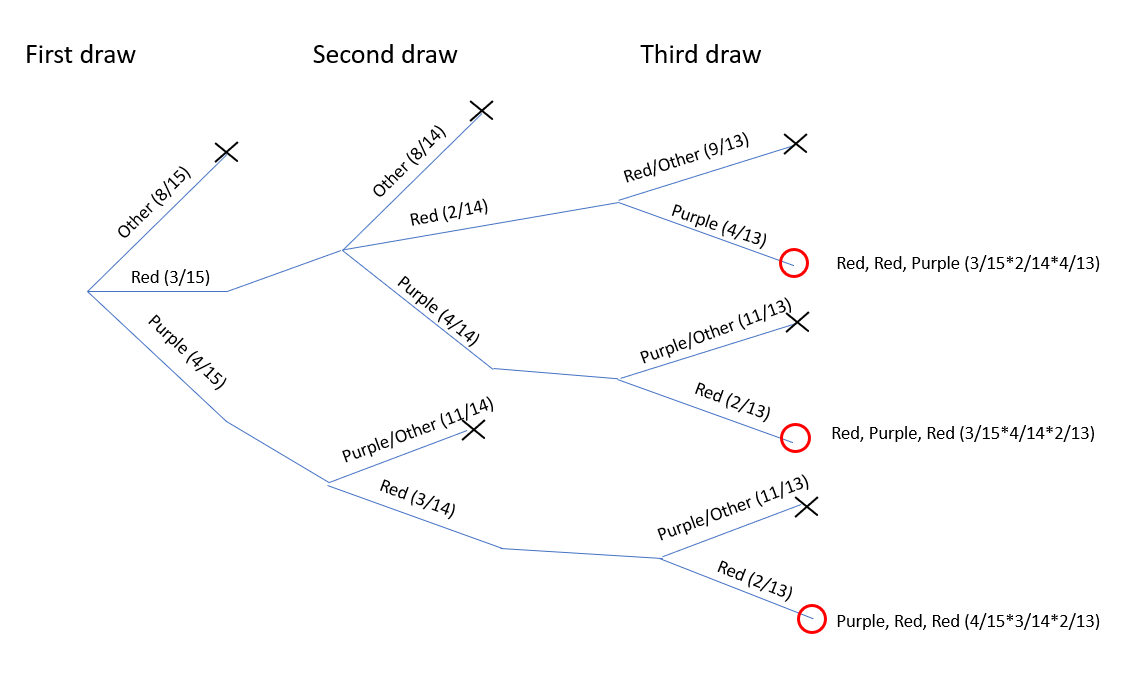
Probability tree illustrating how to calculate sampling without replacement. The red circules indicate branches are successful and the black x's indicate branches that were unsuccessful.

Figure 6.1: Probability tree illustrating how to calculate sampling without replacement. The red circules indicate branches are successful and the black x’s indicate branches that were unsuccessful.

Notice how each path leads to potentially different probabilities at the next branching. In the second draw, the probability of red in the upper pathway is different than the probability of red in the lower pathway. Also note that I’ve combined branches leading to unsuccessful outcomes, and sheared these as soon as it was clear that no success could occur.

After working through the whole tree, we find three successful branches (RRP, RPR and PRR) and see the calculations of their respective probabilities.

In fact, we see that each successful branch has the same probability (because they have to!) of \(24/2730 = \frac{4*3*2}{15*14*13}\). Hence, since these are mutually exclusive, the overall probability is \[P(RRP) = 3*24/2730 = 0.0264\]

6.4.3 Different Ways, Same Results

I want to dive a little deeper into this idea that each successful branch has the same probability.

Again, for this problem, success looks like drawing either (P, R, R), (R, P, R) or (R, R, P).

What’s the probability of the first? (P, R, R) \(=\frac{4}{15}*\frac{3}{14}*\frac{2}{13}\).

What’s the probability of the second: (R, P, R)? \(=\frac{3}{15}*\frac{4}{14}*\frac{2}{13}\).

What’s the probability of the third: (R, R, P)? \(=\frac{3}{15}*\frac{2}{14}*\frac{4}{13}\).

An important takeaway here is that even though the probabilities of each specific draw at each specific point in a given branch are different, when combined, the overall probabilities of each branch are the same. There’s always a 4, 3, and 2 in the numerator and a 15, 14, and 13 in the denominator.

(Note: Don’t make too much out of the exact 4-3-2 pattern in the numerator and that it always decreases. Why not? What would it have been if we were looking for 2 purple and 1 red?)

And since these are disjoint (i.e. only one of these three can happen) we can add these together. More simply, since they’re all the same, just multiply by 3.

6.4.4 Summarizing the Approach

As we’ve seen, when thinking about sampling problems, we can simplify our analysis by using:

“Number of ways” times “Probability of one way”

This general approach works for both sampling with and without replacement, although the “probability of one way” is typically different under the two different sampling schemes.

6.4.5 Guided Practice

Using the Skittle bowl with 15 candies: (4 purple, 3 red, 3 orange, 3 yellow and 2 green)

What is the probability of drawing exactly one green and one orange out of three candies, assuming sampling without replacement?
Sketch out a probability tree to represent this situation
How would this be different if I asked about at least one green and orange?

6.4.6 Link to Conditional Probabilities

There is a link to sampling without replacement and conditional probabilities. Let A and B be successive draws.

\(P(A\ and\ B) = P(B|A)P(A)\)

Meaning, that the probability that I draw both A and B is the probability that I draw B given A was already drawn times the probability that A was drawn.

So, the probability that I draw red and purple is \(P(R\ and\ P) = P(R|P)*P(P) = P(P|R)*P(R)\) but be cautious to ensure you also include the number of ways it could happen.

6.4.7 Simulating without replacement in R

Above we introduced simulation for sampling with replacement. To sample without replacement, we’ll use the same approach, but change (remove) the replace=T parameter.

For example:

sample(c("P", "R", "O", "Y", "G", "B"), 4)

## [1] "Y" "O" "R" "P"

draws four Skittles from a bowl with six. In this case we can’t ever draw duplicate colors. Why not?

If we want a bigger bowl, we need to change the first parameter. We can use the rep() function to create the larger bowl, in this case one with 30 candies.

rep(c("P", "R", "O", "Y", "G", "B"), 5)

##  [1] "P" "R" "O" "Y" "G" "B" "P" "R" "O" "Y" "G" "B" "P" "R" "O" "Y" "G" "B" "P"
## [20] "R" "O" "Y" "G" "B" "P" "R" "O" "Y" "G" "B"

The following code snippet then simulates drawing four candies from a bowl with 30 Skittles of the same colors as above in equal proportions:

sample(rep(c("P", "R", "O", "Y", "G", "B"), 5), 4)

## [1] "R" "Y" "Y" "P"

We’ll come back to simulation work throughout the year, and in particular when we study different probability distributions.

6.5 Ordered vs. Unordered Sets

As a last topic of this chapter, we’ll discuss how to determine the size of ordered vs. unordered sets. In Probability Theory, this is part of a larger topic known as combinations and permutations. Our goal here is simply to introduce the key ideas.

Above we discussed that calculating probabilities often comprises two steps, determining both: (i) how many ways can something occur, and (ii) what is the probability of each way.

To start, let’s review the different between ordered and unordered sets:

Let’s suppose we have 4 aces, one of each suit (\(\spadesuit\), \(\heartsuit\), \(\diamondsuit\), and \(\clubsuit\)). How many ways can you choose 2 of them?

The following table shows all possible outcomes of the two cards:

first ace	second ace
\(\spadesuit\)	\(\heartsuit\)
\(\spadesuit\)	\(\diamondsuit\)
\(\spadesuit\)	\(\clubsuit\)
\(\heartsuit\)	\(\spadesuit\)
\(\heartsuit\)	\(\diamondsuit\)
\(\heartsuit\)	\(\clubsuit\)
\(\diamondsuit\)	\(\spadesuit\)
\(\diamondsuit\)	\(\heartsuit\)
\(\diamondsuit\)	\(\clubsuit\)
\(\clubsuit\)	\(\spadesuit\)
\(\clubsuit\)	\(\heartsuit\)
\(\clubsuit\)	\(\diamondsuit\)

As a first guess, to calculate this without writing down every permutation you might say there are four ways to choose the first ace and then three ways to choose the second ace, and so 4x3=12, which matches.

But do we care about the ordering or not? For example, is (\(\spadesuit\), \(\heartsuit\)) the same as (\(\heartsuit\), \(\spadesuit\))?

If we care about the order and consider results those different, we’re looking for the ordered arrangement. If we don’t distinguish between those, we’re looking for the unordered arrangement.

The specifics will depend on the application. For example, are you asking who’s going, or who got their first? Do you care about which teams make the playoffs, or their ranks? I.e., does the order matter?

6.5.1 The choose Function

Above we’ve discussed how to calculate the size of the ordered set. To determine the size of the unordered set, let’s define what’s known as the choose function:

\[{n \choose r} = \frac{n!}{r!(n-r)!}\] Here \(n!\) stands for n factorial, calculated as: \(n! = n*(n-1)*(n-2)*\cdots * 2 * 1\). Important identities include: \(1! =1\) and \(0!=1\)

The choose function gives us the the number of ways of selecting \(r\) individuals from a group of \(n\) choices if we don’t care about the order.

What we saw above with the aces was that the difference between ordered and unordered pairs is that a number of duplicates exist in the former that don’t in the latter. Therefore the unordered calculation has to remove (i.e. divide out) those duplicates. In fact it’s the \(r!\) in the denominator that cancels out the duplicates.

Back to our aces example, there are \(n=4\) suit choices and we want to select \(r=2\). So,

\[{4 \choose 2} = \frac{4!}{2!(4-2)!} = \frac{24}{2*2} = 6\]

In R we would do this as:

choose(4,2)

## [1] 6

Note that there were 12 pairs in the above table but since each pair is a duplicate, 12/2 = 6, which matches.

6.5.2 Counting and Probability

As a reminder, we can think about probabilities in terms of set theory, where

\(P(A) = \frac{\#\ of\ elements\ in\ A}{\#\ of\ elements\ in\ S}\)

where \(A\) is the event or subset we consider a “success” and \(S\) is the entire set of possible outcomes.

We can use the counting approach described in this section to potentially determine both the numerator and the denominator, although its generally more useful for the denominator.

For example, assume face cards count for 10 points and aces count for 11. What is the probability of getting 21 on two cards (drawing without replacement)?

Let’s tackle the denominator first.. How many ways (unordered) can we draw 2 cards from a deck?

choose(52,2)

## [1] 1326

which is 52*51/2 (where again we divide to get rid of duplicates).

For the numerator, how many of those ways add to 21?

I either need to draw an Ace then 10/Face or a 10/Face then Ace. So there are \(4*16\) ways the first can happen and \(16*4\) ways the second can happen so there are \(128\) ways total. But this is ordered! Since I really want unordered results, I need to divide by two here.

Putting this together, we find the probability of getting 21 on two cards is \(\frac{64}{1326} = 0.0483\).

6.5.3 Guided Practice

How many ways are there to order 6 colored skittles: ROYGBP?
How many ways are there to draw 2 skittles from the same set of 6 colored skittles (ROYGBP) assuming sampling without replacement? How does your answer change if you consider ordered vs. unordered sets?
Assume a bowl has 24 skittles, 4 of each color. How many possible draws of 4 are there (unordered without replacement)? First do this by hand and then use the choose function to confirm the same result.
How many way are there to order a pasta dinner (4 noodle choices, 3 sauce selections and 4 meat options)? What is the probability the customer orders ravioli or sausage or both?

6.6 Review

What we’ve done in this chapter is discuss sampling from a small, known population and learned how to calculate the probabilities of the different outcomes that might occur. We discussed the differences between sampling with and without replacement. We learned visual methods (probability trees) to represent probabilities, which can be particularly useful when sampling without replacement. We saw a few examples of how we can use R to simulate probabilities. Finally, we discussed the differences between ordered and unordered samples and learned about the choose() function.

As we expand our knowledge of statistics, we will switch this order around. In fact, we will take samples from an unknown population and use these samples to make inference about the makeup of that larger population.

6.6.1 Review of Learning Objectives

By the end of this unit you should be able to

Define the terms population, sample, and sample size
Explain the difference between sampling with replacement and sampling without replacement and give examples of when each might be appropriate
Calculate the probability of drawing specific outcomes from small populations of items, using both sampling with and without replacement.
Draw and use probability tree diagrams to represent and solve sampling problems
Explain the formulation of the choose function for different values of \(n\) and \(r\) and calculate using the choose() function in R
Discuss the difference between ordered and unordered sets, and explain why and when ordering is important
Understand how to use R to simulate sampling with and without replacement

6.7 Summary of R functions in this Chapter

function	description
`rep()`	to generate a vector that repeats a certain sequence
`choose()`	to calculate the value of “n choose k”

6.8 Exercises

Note: These are not required and will occasionally be used during class as warm-up exercises or no-stakes quizzes.

Exercise 6.1 In a multiple choice exam, there are 5 questions and 4 possible choices for each question (a, b, c, and d). Nancy has not studied for the exam at all and decides to randomly guess at the answers. What is the probability that she answers:

the first two question correctly and misses the last three?
only the second and fifth questions correctly?
compare your answers to (a) and (b) and discuss and similarities or differences
at least one of the question correctly?
all of the question correctly?

Exercise 6.2 Let’s suppose your professor has 6 different shirts: 1 white, 2 blue, 1 gray, 1 plaid, and 1 brown, and assume he washes them immediately after use, so they’re all available on any day. (He’s apparently not very energy conscious!)

In a given 3 day period, what is the probability that he wears a blue shirt 3 days in a row?
What is the probability that he wears exactly 1 brown and exactly 1 white shirt over the next the 3 days?
What is the probability that he wears a white shirt on at least one of the next three days? (Hint: use the complement rule here.)

Exercise 6.3 Assume you’re drawing 4 candies using sampling with replacement from a Skittle bowl with the following colors: purple, red, orange, yellow, green, blue.

How many ways are there to draw one green, one blue, and either one red or one orange (or both)?
List out the complete table detailing your answer to part (a), or in at least enough detail to convince yourself of your answer to part (a).

Exercise 6.4 For your birthday, you are inviting seven friends to go to an escape room. There will be eight of you in total. Only four people can be in each escape room at a time, so you’ll have two different rooms.

How many ordered ways you can select the people in the first group.
Once you’ve chosen the first group of four people, how many unordered ways are there to choose the second group?
Once you’ve chosen the first group of four people, how many ways are there to order them?
How many unique ways are there to split you and your friends up into the two groups? (Hint: Divide your answer from a by your answer by c.)
What is the probability that you and your best friend are in the same group? (Hint: you do NOT need to enumerate every combination to solve this.)

Exercise 6.5 Using the Skittle bowl with 15 candies distributed as 4 purple, 3 red, 3 orange, 3 yellow and 2 green.

What is the probability of drawing exactly one green, one red and one yellow out of three candies, assuming sampling without replacement?
Sketch out a probability tree to represent this situation.
What is the probability of drawing a rainbow, one of each color assuming drawing 5 candies and sampling without replacement?

Exercise 6.6 Why does sampling with replacement leads to independence between events (successive draws) whereas sampling without replacement does not?

Exercise 6.7 Assume that there are 88 freshman, 90 sophomores, 93 juniors and 89 seniors at EPS.

What is the probability of two randomly selected students both being seniors, assuming sampling without replacement. Then, recalculate assuming sampling with replacement.
What is the difference between your two results?
What does this suggest about when sampling should be done with or without replacement?

Exercise 6.8 You are given an option to choose from a box of dozen (12) Voodoo Donuts containing: Three glazed, two maple bars, three old fashioned, two with colored sprinkles and pink frosting, and two with chopped peanuts on chocolate frosting.

If you randomly choose two (2) donuts without replacement, what is the probability of selecting one maple donut and one donut with peanuts?
If you randomly choose two (2) donuts without replacement, what is the probability that both donuts are the same type?
If you randomly choose three (3) donuts without replacement, what is the probability that you get at least one glazed and one old-fashioned?

Exercise 6.9 If you are dealt three cards, what is the probability that exactly 2 of them match (same value, different suits).

Draw a probability tree that illustrates the situation.

Exercise 6.10 In Dungeons & Dragons, to establish the value of each of a character’s attributes (Strength, Intelligence, Wisdom, Dexterity, Constitution, and Charisma) a player rolls a six-sided die three times and adds the results.

What is the probability that a character’s Strength (one of the attributes) is 15 or greater?
What is the probability that at least 2 of a character’s attributes are 15 or greater?

Exercise 6.11 Paul has 8 cards, and there is a number on each card: 2, 3, 3, 4, 5, 5, 5, 5. Paul draws three cards at random. What is the probability that the sum is odd? Hint: draw a probability tree. (From Barton p310)

Exercise 6.12 The Birthday Problem: Between our two statistics classes, there are about 30 people.

What is the probability that two people selected at random share a birthday?
What is the probability that over all 30 people, at least two people share a birthday?

Exercise 6.13 You roll three die, a red one, a blue one and a white one. What is the probability that the sum of all three dice is at least 15?

(Hint: you can think about this as a sampling with replacement problem, and you might consider sketching a probability tree. What is the result of the first die? Then, given that, what is the second then second die? And then, what value(s) of third die can lead to ``success’’?)

Exercise 6.14 Imagine 5 cards are dealt from a 52 card deck (without replacement) and those 5 cards comprise your “hand”.

What are the possibilities for the number of Hearts in your hand?
What is the probability of there being exactly 2 Hearts in your hand?
Assume you had three Hearts and then are allowed to discard the other 2 cards and draw 2 more. What is the probability the two new cards are both Hearts?

Exercise 6.15 Above we calculated the probability of getting dealt a blackjack (i.e. a sum of 21) hand on your two first cards.

Draw this as a tree to confirm our result.
What is the probability of the dealer NOT also getting the same on her first two cards.

Exercise 6.16 What is the probability of pocket pairs in Texas Hold `em? (Basically, what is the probability of getting two cards that are the same value, regardless of suit, again sampling without replacement.) Attempt to solve this two ways:

think about the total number of possible 2 card hands that exist and how many of those are pairs, and
think about the what the first card could be and then what the second card could be, and probabilities of each that make a pair.