Chapter 15 Intro to Simulation Based Inference
15.1 Overview
The purpose of this lab is to introduce another approach to hypothesis testing that relies less on assumptions about the underlying data and more on simulation of the null distribution. Generally this approach falls under what is known as Simulation Based Inference.
In our Testing the difference in proportions screencast we used the following data:
| preference | video games | sports | total |
|---|---|---|---|
| fr/so | 28 | 24 | 52 |
| jr/sr | 27 | 32 | 59 |
which game us an estimated \(\hat p_1\) for the preference of video games for underclassmen as:
## [1] 0.5384615We also found that overall there were 55 out the the 111 people sampled who preferred video games.
Our previous question was “Is there a statistically difference in preference between under- and upper-classmen?” We relied on the CLT and built our null distribution based on that.
However, as alluded to above, there’s another way…
15.2 What if we had Random Assignment?
If those 55 responses of video games and 56 responses of sports had been randomly assigned to the students in the two groups (i.e. under- vs upper- classmen), how likely is it to see the result we did?
In other words, is it reasonable that our observed result of \(\hat p_1 = \frac{28}{52} = 0.538\) would arise from randomness alone?
We can answer this pretty easily in R using simulation. Let’s take those 55 video game and 56 sports responses and randomly assign them to people in the two groups, and then see what happens. In particular, we’ll build our null distribution via simulation instead of using our equations from the CLT.
15.3 Simulating a Single Random Response
First, let’s create a vector of 55 video games and 56 sports responses, and the (randomly) shuffle them:
##   [1] "V" "V" "V" "V" "V" "S" "S" "V" "V" "V" "S" "S" "V" "V" "S" "V" "S" "V"
##  [19] "V" "V" "S" "S" "S" "S" "S" "S" "V" "S" "S" "S" "V" "S" "V" "V" "S" "S"
##  [37] "S" "S" "V" "S" "V" "V" "S" "V" "S" "S" "S" "S" "V" "V" "V" "V" "V" "S"
##  [55] "S" "V" "S" "V" "S" "V" "S" "V" "S" "S" "V" "V" "V" "V" "S" "V" "S" "V"
##  [73] "V" "S" "S" "S" "V" "V" "S" "V" "V" "S" "S" "V" "S" "V" "S" "S" "V" "S"
##  [91] "S" "V" "V" "S" "V" "V" "S" "V" "V" "S" "S" "V" "S" "S" "S" "S" "S" "V"
## [109] "V" "S" "V"
Now, let’s take the first 52 (although that we could take any 52) and assign those to the Fr/So (under-classmen) group. In such a random sample, what is our estimate of \(\hat p_1\)?
rand <- sample(pref)            ## randomly shuffle the group
underclass <- rand[1:52]        ## take the first 52 for underclass
uc_count <- length(which(underclass=="V"))  ## the # of video game responses
p1.hat <- uc_count/52        ## what proportion video games
cat("one random estimate of p1-hat:", round(p1.hat, 3), "\n")
## one random estimate of p1-hat: 0.538Run this chuck multiple times to get a feel for the variability that exists in this random value.
15.4 Knowledge Check
Can someone explain what this random value represents?
15.5 Simulating our Null Distribution
Now let’s use this approach to build our null distribution. The idea here is that if we reshuffle and sample many, many times these results should give an indication of what is likely just as the result of random assignment.
Here’s my code to create the random distribution, which I then plot as a histogram.
a <- vector("numeric", 10000)

for (i in 1:length(a)) {
  rand <- sample(pref)            ## randomly shuffle the group
  underclass <- rand[1:52]        ## take the first 52 for underclass
  uc_count <- length(which(underclass=="V"))  ## the # of video game responses
  p1.hat <- uc_count/52        ## what proportion video games
  a[i] <- p1.hat
}

hist(a, breaks=24, main="simulated distribution of p1.hat", xlab="p1.hat", freq=F)
abline(v=55/111, col="blue1")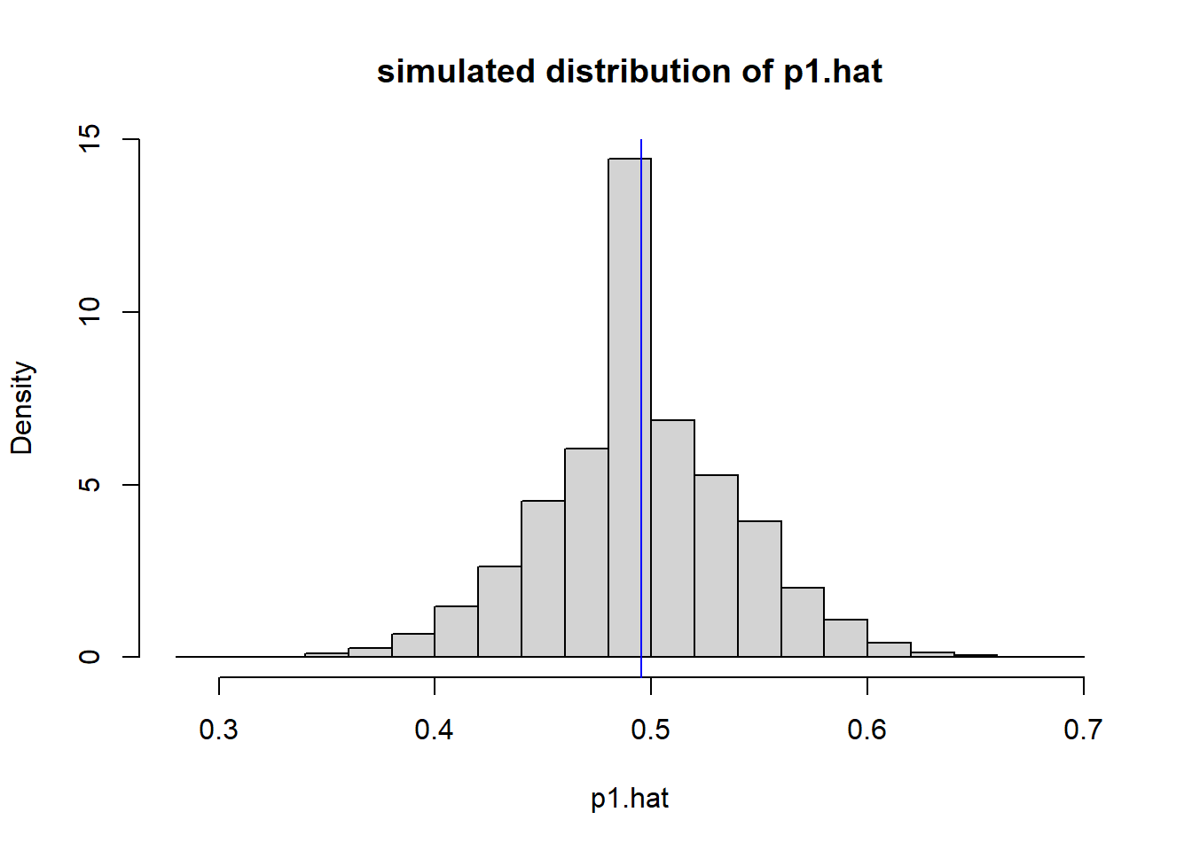
The blue line here is the overall value of \(p\), i.e. the percent that prefer video games regardless of class. As shown below, the pooled estimate of \(p\) and the mean value of the distribution are basically the same.
## Mean of the simulated distribution: 0.496## pooled estimate of p: 0.495What this histogram shows, is the distribution of \(\hat p_1\) IF we randomly distribute the 55 video responses between the two groups.
Based on this, we can now ask “How likely (or unlikely) was our observed response, again assuming the results were random assigned to the two groups (i.e. no difference)?”
hist(a, breaks=24, main="simulated distribution of p1.hat", xlab="p1.hat", freq=F)
abline(v=obsvd.p1.hat, col="red")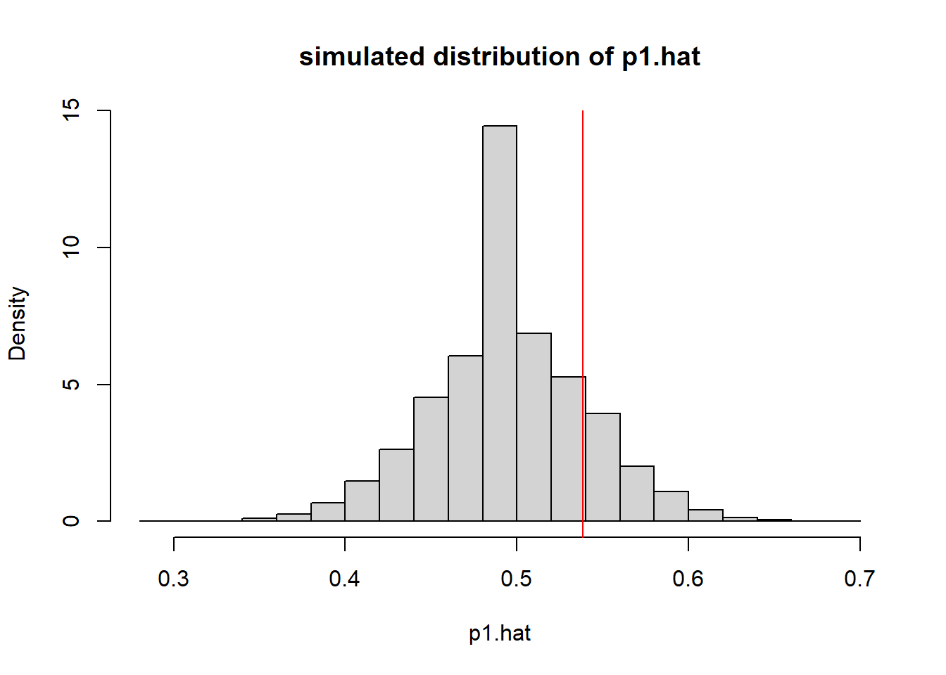
I think we see this isn’t really that extreme at all. We’d need to be below 0.4 or above 0.6 or so before we thought that our observed value was really unlikely just based on randomness alone. So, in this case, it seams reasonable to that we fail to reject our \(H_0\) of no difference in the proportion who favor video games vs. sports between the groups (under- vs upper- classmen).
And mote that we did this all without ever appealing to the CLT or parameterizing the null distribution.
15.6 Summary
Our previous null hypothesis was \(H_0: p_1 = p_2\). Is this different? By randomly assigning the “V” and “G” to each group, we’d expect (on average) both under- and upper- classmen to see the overall proportion \(p = \frac{55}{111}\). So, in fact our null hypothesis is the same when using simulation based inference. The only difference is how we build our null distribution and what assumptions we’re making (or in this case, not making).
FWIW, this type of approach is a bit on the “cutting edge” approach to teaching statistics.