Chapter 12 Students T-test
12.1 Introduction to Student’s t-test
Actually our story today is about Guinness beer. And really about this guy, William Gosset, at one time the head brewer at Guinness:
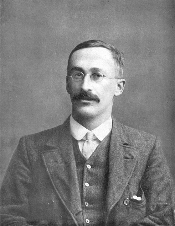
Figure 12.1: William Sealy Gosset - who developed the Student’s t-test
But I’m getting ahead of myself…
In this chapter we will looking at continuous data (that is possibly Normally distributed) and importantly, here we will relax the assumption about needing a prior estimate of \(\sigma\). So, we will no longer assume the population standard deviation is known. But that means we can no longer rely on the CLT and so our Null distribution will no longer be Normal. So what will we use instead?
12.1.1 Learning Objectives
By the end of this chapter students should be able to:
- Describe when a t-test is appropriate
- Discuss the key differences in running a hypothesis test using a t-test (compared with a one sample test assuming \(\sigma\) is known)
- Explain how to use the t-distribution to create a confidence interval
In this chapter we are going to switch the order slightly and discuss how to run the hypothesis testing first and then follow that with how to create confidence intervals.
12.2 Hypothesis Testing using the t-distribution
Let’s again work through an example….
New York is known as the “city that never sleeps.” Is that true? Is the average amount sleep for New Yorkers different than the rest of America?
Suppose you know the average person in America gets 6.8 hours of sleep per night, is there a statistically significant difference between New Yorkers and the rest of America?
Similar to our previous analysis, this is a two-sided test where our null hypothesis will be that there is no difference between New Yorkers average sleep and the rest of America, which we will write as \(H_0:\mu = 6.8\). The alternate hypothesis (for a two-sided test) is that there is some statistically significant difference, or \(H_A:\mu \ne 6.8\).
And let's assume we will poll \(n=25\) people and as before we will test this at \(\alpha=0.05\).
Remember our hypothesis testing process:
- Decide on our null and alternative hypothesis
- Choose our \(\alpha\) level (typically set at \(\alpha=0.05\))
- Determine our null distribution and calculate the critical value(s)
- Collect the data and calculate the test statistic
- Compare the test statistic to the critical value(s) and draw our conclusion
- Calculate the p-value of the test
So we have already done the first two steps here, however this is where things start to change. In fact, our null distribution, test-statistic, and standard error will all be a little different than before.
12.2.1 Normal vs. t Distribution
When we previously calculated our null distribution for continuous data, we needed to know the population standard deviation, \(\sigma\), and then used that, along with our sample size to determine the standard error.
However here, we are NOT assuming \(\sigma\) is known. This is typically the more realistic scenario. As a substitute for this, we will end up using \(s\), the standard deviation of our sample itself. (Note that we didn’t previously consider this value.)
Not knowing \(\sigma\) causes a bit of a problem, and the result is that we can no longer use the Normal distribution for our null and instead have to use what is known as the "Student’s t-distribution".
Let’s compare the standard Normal to the Student’s t-distribution. What is the same? What is different?
x<-seq(from=-3.5,to=3.5, by=0.1)
plot(x, dnorm(x), type="l", col="red", ylab="probability")
lines(x, dt(x, df=12), lty=2, col="blue")
legend(1.75, 0.35, legend=c("Normal", "Student's t"), lty=c(1, 2), col=c("red", "blue"))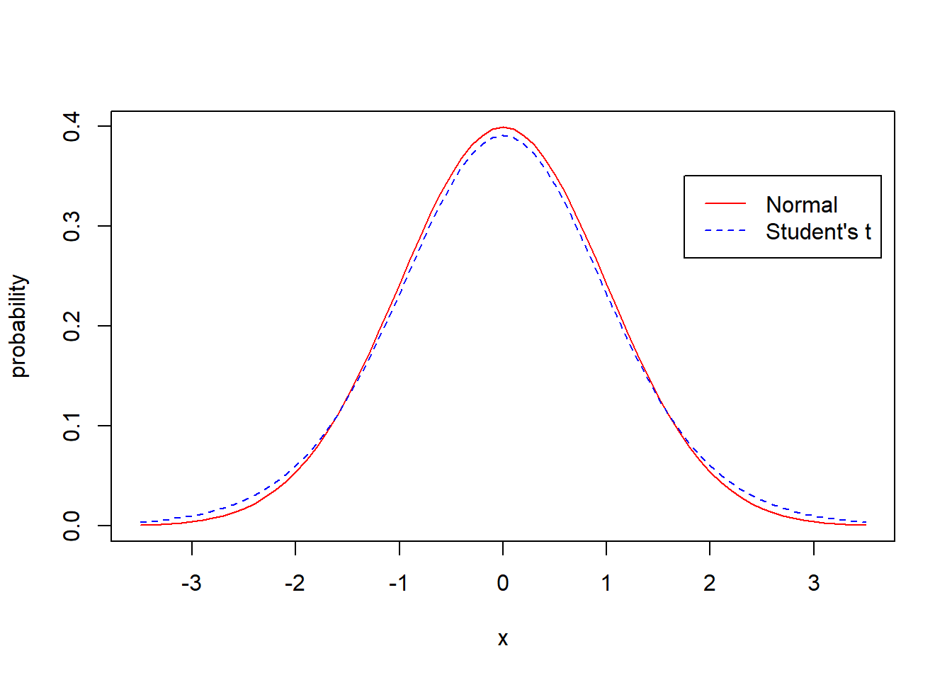
Obviously they’re similar, but not exactly the same. How would you describe the differences, and be specific?
What you probably observe is that the t-distribution puts a little more probability in the tails and has a little less probability in the center. This is the result of the uncertainty of not knowing \(\sigma\). Overall we are a bit less certain and so the distribution spreads out.
You may also have noticed that I’ve centered both the Normal and t-distribution around 0. This will be important in what follows.
12.2.2 Parameters of the t-Distribution
When dealing with the t-distribution, there are two important points to consider. First, it’s always centered at zero (similar to the standard Normal). Second, it only has 1 parameter, the so-called degrees of freedom, \(df\) (which is a term we will start to encounter more often as we go forward). For a t-distribution, \(df=n-1\) where \(n\) is the number of samples we take.
But how then do we incorporate \(s\), the sample standard deviation? More on that in a moment.
12.2.3 The t-Distribution in R
Also, since this is a new distribution to us, the typical suite of R commands is available to us:
dt()returns the probability density (use only for plotting!)pt()returns the probability above or below a certain valueqt()returns the t-value associated with a given probabilityrt()generates a set of random numbers from a distribution
The first letter of the function gives away its usage. And we’ll use these exactly as we did the corresponding Normal functions.
More information on these functions is available on the help page in R: e.g. ?dt.
12.2.4 Why is it called a Student’s t?
The following article gives some interesting context about the development of the t-distribution:
https://medium.com/value-stream-design/the-curious-tale-of-william-sealy-gosset-b3178a9f6ac8
12.2.5 Parameterizing our Null Distribution
Above we were looking at the average sleep of NYers compared to the rest of America.
So, how do we parameterize our null distribution for this example? Since we are taking a sample of \(n=25\) people, our null distribution will be a t-distribution with \(df=24\) degrees of freedom. (Again, \(df=n-1\).) And that’s it!
Next, assuming \(\alpha=0.05\) and a two-sided test, we can then determine our critical values using:
## [1] -2.063899## [1] 2.063899You might note these values are slightly wider than our \(\pm 1.96\) that we’d expect from a standard Normal (again because less probability is located in the middle and more probability is put in the tails, the critical values push out.)
And here is a plot of the null distribution with the critical values:
x<-seq(from=-3.5,to=3.5, by=0.1)
plot(x, dt(x, df=24), type="l", col="blue", ylab="probability")
abline(v=-2.064, col="red")
abline(v=2.064, col="red")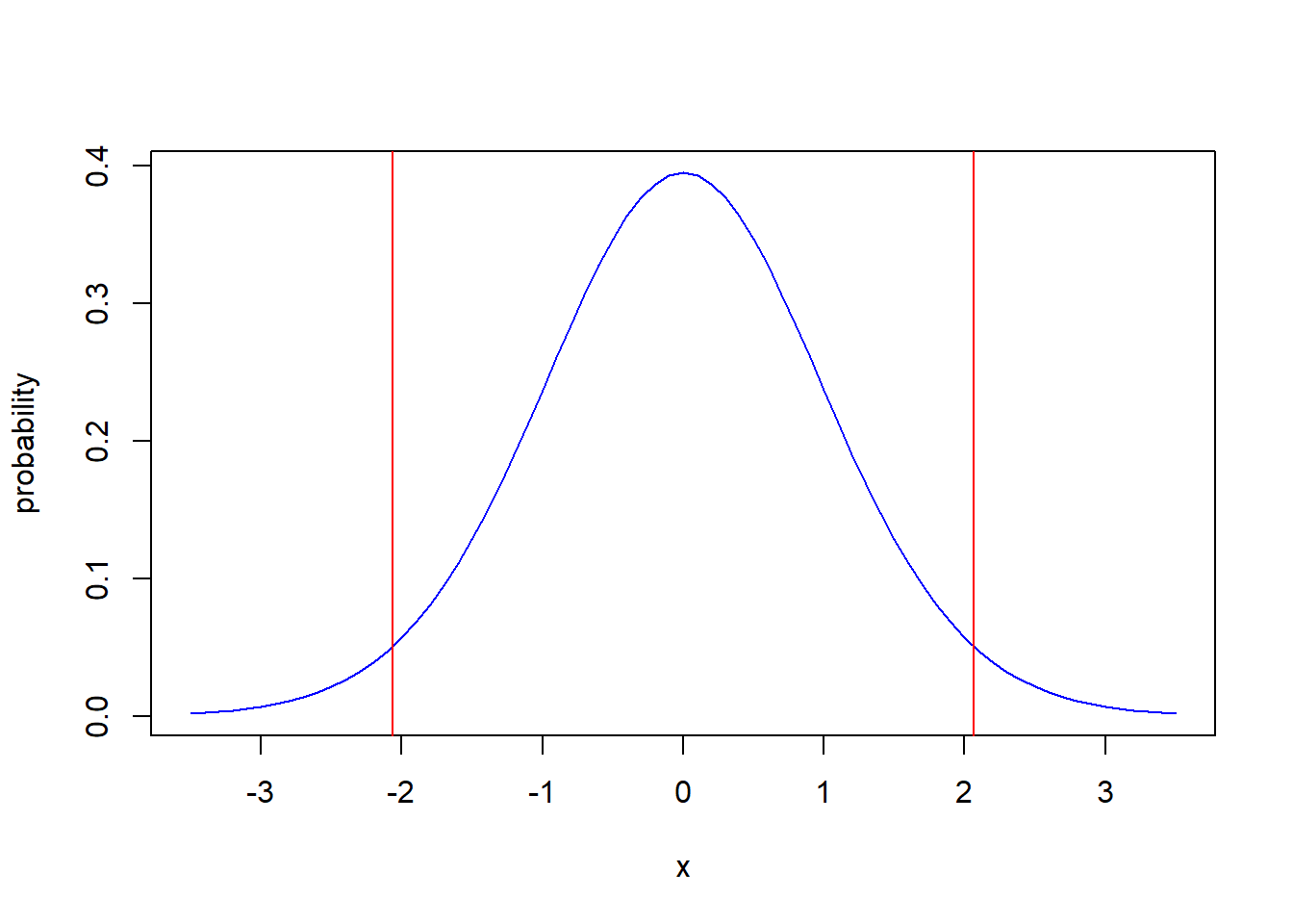
12.2.6 Collecting our Data
Now that we have found our null distribution and critical values, our next step would be to go collect data. Above we discussed we would poll \(n=25\) (random) New Yorkers about how many hours they sleep per night. Assume we did this and found the following results (statistical summaries):
| \(n\) | \(\bar X\) | \(s\) | min | max |
|---|---|---|---|---|
| 25 | 6.51 | 0.77 | 5.17 | 9.78 |
12.2.7 Our Test Statistic
Next, we need to calculate our test statistic to compare it against our null distribution.
IMPORTANT: Our distribution is centered at 0, so it doesn’t make sense to look at only \(\bar X\). Moreover, we know we need to incorporate \(s\) somehow.
You may remember that we could shift a Normal distribution to the standard Normal by using the z-score as \(Z = \frac{x-\mu}{\sigma}\). In this case we’ll do something similar, using a “t-score”:
\[T = \frac{\bar X - \mu}{SE}\] where \(\bar X\) is the mean of the data we collect, \(\mu\) comes from our null hypothesis and SE is the standard error of the observed data.
How do we find the standard error here if we don’t know \(\sigma\)? Similar to what we did previously, we will use \[SE = \frac{s}{\sqrt{n}}\]
where \(\sigma\) has been replaced by \(s\).
Hence, using the data from our NY sleep example, let's first calculate the standard error as: \[SE = \frac{0.77}{\sqrt{25}} = 0.154\]
Then, we can incorporate this into our test statistic calculation to find:
\[T = \frac{6.51 - 6.8}{0.154} = -1.883\]
Now the question we are really asking is, how likely is it to see a value as extreme as \(-1.883\) given a T-distribution with 24 degrees of freedom?
Let’s look back at our critical values: -2.064 and 2.064. It should be obvious that a test statistic as large as \(-1.883\) will fall inside these critical values. Hence, we know we will fail to reject \(H_0\).
Of course let’s also evaluate how likely it is to see a value as extreme as \(-1.883\) given a t-distribution with 24 degrees of freedom. To calculate our p-value we will use the pt() function as (remembering this is a two-sided test):
## [1] 0.07187646This is a small number, but it is just above \(\alpha=0.05\) and so we’d fail to reject our null hypothesis and conclude that there is not a statistically significant difference between the average amount of sleep New Yorkers get compared to the rest of the country.
Of note, the average of our sample was less than the mean value for Americans, but there just wasn’t enough evidence to conclude that the sample value is “statisically” different.
12.3 Summarizing the differences between one sample tests
Below I’ll present a table summarizing the details of in each step, but for now, the key differences introduced above (as compared to our test when \(\sigma\) is known) are:
- t-distribution with \(n-1\) degrees of freedom instead of Normal distribution
- use of
qt()to find the critical values
- Standard error uses \(s\) instead of \(\sigma\)
- use \(T=\frac{\bar X-\mu}{SE}\) instead of \(\bar X\) as the test statistic
- use of
pt()to find the p-value
12.3.1 Guided Practice
Researchers interested in lead exposure due to car exhaust sampled the blood of 52 police officers subjected to constant inhalation of automobile exhaust fumes while working traffic enforcement in a primarily urban environment. The blood samples of these officers had an average lead concentration of 124.32 \(\mu\)g/l and a SD of \(s=37.74\) \(\mu\)g/l; a previous study of individuals from a nearby suburb, with no history of exposure, found an average blood level concentration of 35 \(\mu\)g/l.
- Write down the hypotheses that would be appropriate for testing if the police officers appear to have been exposed to a different concentration of lead.
- Test the hypothesis that the downtown police officers have a different lead exposure than the group in the previous study. Interpret your results in context.
12.4 Using Built-in Functions and Scripts in R
12.4.1 Using t.test() in R
R (being a statistical software package) has a built in function, t.test() that makes this work pretty easy for us if we have all the data.
For example, let’s suppose we had the following data on hours of sleep (similar to our original example above) but now from a sample of Seattle:
sea <- c(7.4, 6.4, 8.2, 7.1, 6.9, 7.8, 7.2, 7.6, 7.5, 7.0, 7.8, 8.8, 7.6, 8.5, 8.1, 6.5, 9.1, 8.1, 9.4, 7.7, 6.6, 7.8, 8.4, 7.5, 8.2)
mean(sea)
## [1] 7.728## [1] 0.7716433If we want to evaluate the null hypothesis that this comes from a distribution with \(\mu= 7.1\) (different from what we asked above), we would simply call:
##
##  One Sample t-test
##
## data:  sea
## t = 4.0692, df = 24, p-value = 0.0004423
## alternative hypothesis: true mean is not equal to 7.1
## 95 percent confidence interval:
##  7.409481 8.046519
## sample estimates:
## mean of x
##     7.728
Note that the default is to run a two-sided test at \(\alpha=0.05\).
Of key importance, notice the p-value given as 0.0004423 (on the 5th line of the output). Since this is less than \(\alpha=0.05\) we will reject \(H_0\).
To confirm the calculation of the test statistic here, given above as t = 4.0692 (also listed on the 5th line of the output), note:
# Setup the mean value
mu <- 7.1

# How many observations?
n <- length(sea)

# Calculate and return the test statistic
(mean(sea)-mu)/(sd(sea)/sqrt(n))
## [1] 4.069238which matches.
The advantage of using the t.test() function is that we only have to pass R (i) the data and (ii) the hypothesized population value \(\mu\) and R does everything else for us. Nice, right?
More information on the t.test() function is available in the R help. In particular, to run a one sided test, you should set the alternative="less" or alternative="greater" parameter. Again, the default is “two.sided”. You could also change \(\alpha\) if desired.
12.4.2 Writing our own Script
If we don’t have the all data, but instead just the summary statistics, we can still do this pretty easily by writing our own script.
Here again is the summary of our NY sleep data:
| \(n\) | \(\bar X\) | \(s\) | min | max |
|---|---|---|---|---|
| 25 | 6.51 | 0.77 | 5.17 | 9.78 |
The following script runs a t-test based on only the summary data.
#------------------------------------------------------------------------------#
# Load in our summary data from our test #
n <- 25        # the number of samples
mu <- 6.8      # the null hypothesis
x.bar <- 6.51  # the observed mean
s <- 0.77      # the observed standard deviation

#------------------------------------------------------------------------------#
# Calculate the key results and print out the conclusion #
my.SE <- s/sqrt(n)
cat("standard error:", round(my.SE, 3), "\n")
my.t <- (x.bar-mu)/my.SE
cat("test statistic", round(my.t, 3), "with", n-1, "degrees of freedom.\n")
cat("critical values:\n")
cat("  lower:", round(qt(0.025, n-1), 3), "\n")
cat("  upper:", round(qt(0.975, n-1), 3), "\n")

if (my.t > 0) {
  my.p <- 2*pt(my.t, n-1, lower.tail=FALSE)
} else {
  my.p <- 2*pt(my.t, n-1)
}
cat("p-value:", my.p, "\n")
#------------------------------------------------------------------------------#
As a reminder, the cat() function prints out information to the screen.
If you modify the first few lines, you can change the null hypothesis and details of the data.
12.5 Inference for the t-distribution
What if instead of running a hypothesis test, we simply wanted to create a confidence interval around the true value of \(\mu\)? We would proceed as we did in the last chapter, but of course this time using the t-distribution.
Sticking with our sleep data,
| \(n\) | \(\bar X\) | \(s\) | min | max |
|---|---|---|---|---|
| 25 | 6.51 | 0.77 | 5.17 | 9.78 |
let’s calculate a 90% confidence interval on the true value of the mean for New Yorkers.
For a 90% confidence interval we want 5% of the distribution outside of the bounds. So, based on a t-distribution we will first find the values that contain the middle 90% of the t-distribution itself, then we will use those to determine the interval on \(\mu\).
For the bounds of the t-distribution we will use:
## [1] -1.710882## [1] 1.710882Next, we need to relate these values back to \(\mu\). To do this, we will “unwind” the test statistic.
Our test statistic was \(t=\frac{\bar X-\mu}{SE}\), so solving this for \(\mu\) we find \[\mu = \bar X + t*SE\]
where the values of \(t\) come from the above qt() function call. Note we aren’t technically calculating \(\mu\) here, but a quantile of the true distribution.
Plugging these values in, we find the lower bound on \(\mu\) to be:
## [1] 6.246524And similarly the upper bound to be:
## [1] 6.773476So, the true average of New Yorker’s sleep likely falls between \(6.24\) and \(6.77\) hours. The specific interpretation of the confidence interval in this case is the same as in the previous chapter.
12.5.1 The General Form
For confidence intervals from the t-distribution we will use the following general formula:
\[\bar X \pm t_{df, \alpha/2} * SE\] where:
- \(\bar X\) is our estimate of the mean,
- \(t_{df, \alpha/2}\) is the multiplier for our specific t distribution describing what percent of the distribution we want, and
- \(SE\) is our estimate of the standard error.
As we observed above, the t-distribution is centered around 0 so using qt() on probabilities below 0.5 results in a negative value and using it on probabilities above 0.5 result in a positive value. Also note that the \(t\) values are symmetric around 0, which means we only really need to calculate it once.
Because of this, the following intervals are equivalent:
- \(\{- t_{df, \alpha/2}, + t_{df, \alpha/2}\}\)
- \(\{t_{df, (1-\alpha/2)}, t_{df, \alpha/2}\}\)
Referring back to the example above, how would we find the \(t\) value (the multiplier) for a 99% confidence interval?
We would set \(\alpha=0.01\), and so find \(\alpha/2 = 0.005\), leading us to calculate the \(t\) value as (assuming \(df=24\)):
## [1] -2.79694Hence a 99% confidence interval on the true mean (again assuming \(df=24\)) would be: \[\{\bar X -2.797 * SE, \bar X +2.797 * SE\}\]
12.6 Summary and Review
The Student’s t test is used for continuous data, when we don’t know the population’s standard deviation. The main difference between this test is that it utilizes the t distribution instead of a Normal distribution.
The following table highlights the differences between using a t-test or a Normal one sample test, particularly where we have converted the null distribution for the Normal test to the Standard Normal:
| item | Student’s t test | Hypothesis testing if \(\sigma\) known |
|---|---|---|
| Null and Alternative | \(H_0: \mu = \mu_0\), \(H_A: \mu \ne \mu_0\) | \(H_0: \mu = \mu_0\), \(H_A: \mu \ne \mu_0\) |
| SE | \(\frac{s}{\sqrt{n}}\) where \(s\) is the sample standard deviation and \(n\) is the number of samples | \(\frac{\sigma}{\sqrt{n}}\) |
| test statistic | \(\frac{\bar X-\mu}{SE}\) | \(\frac{\bar X-\mu}{SE}\) |
| Null distribution | \(t(n-1)\) (a t distribution with n-1 degrees of freedom) | \(N(0,1)\) |
| critical values (at \(\alpha = 0.05\)) | qt(0.025, n-1), qt(0.975, n-1) |
\(\pm 1.96\) |
| p-values | pt(\(\frac{\bar X-\mu}{SE}\), \(n-1\)) |
pnorm(\(\frac{\bar X-\mu}{SE}\),\(\mu=0\), \(\sigma=1\)) |
where \(\mu_0\) is some hypothesized value.
Note: The test statistic given for the case with \(\sigma\) known may be different than expected. What I’ve shown is \(\frac{\bar X-\mu}{\sigma}\) and this is then compared against \(N(0,1)\). As we’ve shown, particularly when we were discussing z-scores, this is equivalent to comparing \(\bar X\) to \(N(\mu, \sigma)\).
Said differently, if \(X\sim N(\mu, \sigma)\) then \(\frac{(X-\mu)}{\sigma} \sim N(0,1)\).
12.6.1 Review of Learning Objectives
By the end of this chapter students should be able to:
- Describe when a t-test is appropriate
- Discuss the key differences in running a hypothesis test using a t-test (compared with a one sample test assuming \(\sigma\) is known)
- Explain how to use the t-distribution to create a confidence interval
12.7 Exercises
Exercise 12.1 A study suggests that the average college student spends 10 hours per week communicating with others online. You believe that this is an underestimate and decide to collect your own sample for a hypothesis test. You randomly sample 30 students from your dorm and find that on average they spent 11.5 hours a week communicating with others online, with a sample standard deviation of \(s=3.5\).
- Write down the hypotheses that would be appropriate for testing if the students spend more time on line.
- Test the hypothesis that students spend more time on line than the previous study suggested. Interpret your results in context.
Exercise 12.2 Create a plot of the t-distribution for 5 degrees of freedom. Then overlay plots of 10, 20, 30 and 40 degrees of freedom. Finally overlay a standard Normal plot. Describe what you see, and in particular where do you observe the largest differences between a normal and t-distribution?
Exercise 12.3 A particular model of hiking boots is known to have an average lifetime of 15 months. Someone in R&D (research and development) claims to have created a less expensive, but just as long lasting boot. This new boot was worn by 20 individuals and the data for how long they lasted (in months) is shown below. Is the designer’s claim of a 15 month lifetime supported by the trial results? Evaluate at an alpha (significance) level of 0.05. You can do this by hand or using the t.test() function in R, or better yet, do it both manually and using t.test() and compare the results.
boot <- c(6.23, 16.10, 18.03, 15.05, 29.35, 21.20, 20.48, 14.80, 8.20, 24.39, 18.26, 17.29, 12.48, 9.69, 15.34, 6.58, 11.31, 15.16, 21.74, 18.71)
Exercise 12.4 A 95% confidence interval for a population mean, \(\mu\), is given as (18.985, 21.015). This confidence interval is based on a simple random sample of 36 observations. Calculate the sample mean (\(\bar X\)) and standard deviation (\(s\)). Use the t-distribution in any calculations.
Exercise 12.5 Researchers were interested to evaluate if meditation can help reduce anxiety. They measured anxiety using a scale which rates people between 0 and 56. A lower score indicates less anxiety, and assume the average score is in the population is 20. Ten subjects underwent a daily mediation program for four weeks and then were scored on the above scale. Their results are given in the R object below.
Run a hypothesis test to see if meditation seems to reduce anxiety compared to the overall population. (Hint: if you use the t.test() function, make sure to set the alternative= parameter appropriately.)
Exercise 12.6 The above script runs a two sided test. How would you change it to run a one-sided test?
Exercise 12.7 The average time for all runners who finished the Cherry Blossom Race in 2006 was 93.29 minutes (93 minutes and about 17 seconds). Using data from the 2017 Cherry Blossom Race we want to determine whether runners in this race are getting faster or slower, versus the other possibility that there has been no change.
The sample mean and sample standard deviation of the sample of 100 runners from the 2017 Cherry Blossom Race are 97.32 and 16.98 minutes, respectively. Run a hypothesis test using a t-distribution to evaluate if there is a statistically significant difference in average times. What do you conclude? What is your p-value? Create a plot of the null distribution and indicate where the critical values and test statistic are.
Exercise 12.8 Researchers take a small sample of a new variety of barley to evaluate its yield (in bushels per acre). The following table summarizes their sampling results.
Run a hypothesis test at \(\alpha=0.05\) to evaluate if there is a significant difference between the new variety and the existing one, which yields an average of 70 bushels per acre. What do you conclude?
| \(n\) | \(\bar X\) | \(s\) |
|---|---|---|
| 12 | 68.4 | 2.5 |