Chapter 11 One Sample Hypothesis Testing and Inference
11.1 Overview
In this chapter, and most of the rest of the course, we will switch our focus to applications of statistical methods where we can take data samples and use those to make reasonable estimates about a larger population. We will begin here by introducing concepts of statistical inference and one sample hypothesis testing.
So far in this course we’ve assumed we knew the parameters of our distributions, such as \(p\) for the Binomial distribution or \(\mu\) and \(\sigma\) for the Normal distribution. However, we usually don’t. Maybe the population is too big to fully measure. Or maybe we have two different groups and we want to evaluate if their distributions (typically means) are the same.
In this and the following chapters we will learn methods about how to estimate the population parameters from a sample, and how to perform statistical tests to evaluate how likely a parameter is a certain (prespecified) value. The first (“estimation”) uses a process known as statistical inference and the second (“testing”) occurs via hypothesis testing.
We will look at a range of situations where this is applicable, including one or two samples, whether we’re measuring discrete or continuous data, and under different conditions, such as whether certain information is known or not, such as the population variance.
To start, we will attempt to build an understanding of sampling variability.
11.2 Samples, Populations and Uncertainty
Download the Gettysburg Address R notebook from Canvas.
The goals of this exercise are to get comfortable with the concepts of samples vs. populations and the idea of how much uncertainty (error) exists in a sample. We’ll also learn what standard error is and one method to calculate it.
11.3 Inference for Proportions
11.3.1 Learning Objectives
In this section we will be introducing statistical inference for the binomial distribution, and in particular we will attempt to estimate the value of \(p\), the only parameter.
This commonly occurs during election cycles. We don’t know the true value of \(p\), so we use polling to estimate it. But how good is this estimate? And can we use our estimate to quantify the range where the true value likely lies? We’ll find answers to those questions below.
In all previous applications of the Binomial distribution we assumed \(p\) was known. But how is it knowable? We’d have to ask the whole population, right? That isn’t typically feasible. Instead, what we usually do is take a sample of the population, calculate the best estimate of \(p\), which we’ll term \(\hat p\), and then make inference about where the true value of \(p\) probably lies.
The learning objectives of this section are that you can:
- Calculate \(\hat p\) from our sample, which will be our best estimate of the true population parameter, \(p\)
- Understand what standard error means and how to calculate it for the binomial distribution. Explain how standard error and standard deviation are different from one another.
- Create a confidence interval for the true value of \(p\), and explain what it really means
- Describe what a “margin of error” is and how it relates to confidence intervals for polling data
11.3.2 Sampling a Known Population
Suppose we wanted to sample Washington’s 8th Congressional District. In 2020 about 412,000 people voted and Kim Schrier won with 51.7% of the vote (https://ballotpedia.org/Kim_Schrier).
Inspect the following code:
The pop variable is huge, and contains the whole population. Because its a simulation, here we assume we know the true value of \(p=0.517\). However, typically we don’t, and that’s part of the value of simulation.
Here are our questions:
- If we take a sample of the whole population and estimate \(\hat p\), how close is it to the true value of \(p\)?
- Based on that and \(n\) (our sample size), what can we say about the true value of \(p\)? How often can we correctly estimate it?
Pause here. Our whole population (412k people) is huge! We typically can’t poll everyone. But we can poll a sample. And we want to use our sample results to make inference about the population.
So, how do we proceed? Specifically how do we estimate \(\hat p\)? There’s a lot of technical detail behind this, which I won’t cover, but the so-called maximum likelihood estimator (MLE) of \(p\) is \(\hat p = \frac{Y}{n}\), where \(Y\) is the number of successes in our poll divided by the total number \(n\) of people we poll. If we took a poll of 100 people and we found 55 people supporting Kim Schrier, then we’d set \(\hat p = \frac{55}{100} = 0.55\).
11.3.3 Run the Simulation Once
To proceed we are going to simulate polling a sample of voters from our large population.
- To simulate 1 value of \(\hat p\), run the following code:
## Set the sample size
n <- 384
## Draw a sample from the larger population
y <- sample(pop, n, replace=T)
## Calculate and print out p.hat
p.hat <- sum(y)/n
p.hat
## [1] 0.5416667What does this do? It simply finds one estimate of \(\hat p\), in this case 0.5416667.
Ok, that is interesting, but since it is only based on one sample it doesn’t tell us too much. But at this point we can ask:
- How close is \(\hat p\) it to \(p\)? What’s the error (difference) between the two?
Here we see the difference is 0.0246667.
Do this a couple of times and then let’s report out some of your values and write them on the board. What do we see?
(The answer should be that there is a lot of variation, that few if anyone got it exactly right, and that some values aren’t very close.)
11.3.4 Knowledge check:
- What is \(p\)? What is \(\hat p\)? Why are they likely different?
- Why is \(\hat p = \frac{Y}{n}\) a good estimate of \(p\)?
11.3.5 Run the simulation many times
Ok, now, we’re going to run the simulation many, many times to see the distribution of \(\hat p\).
## Set the sample size
n <- 384

## Create a storage vector for our results
my.dat <- vector("numeric", 10000)

## Run a for() loop to estimate 10000 p.hat values
for (i in 1:length(my.dat)) {
  my.dat[i] <- sum(sample(pop, n, replace=T))/n
}

## Plot the distribution of results
hist(my.dat)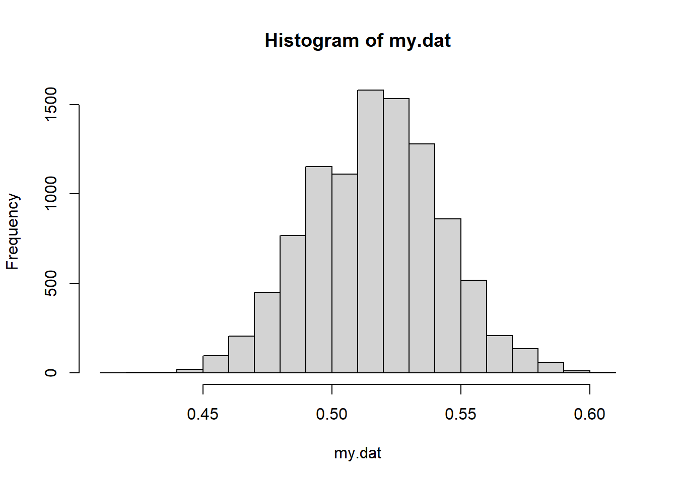
This simulates 10,000 values of \(\hat p\) for \(n=384\). What do you know/notice/wonder?
Now let’s calculate the mean and standard deviation of the simulated data.
## [1] 0.5169844## [1] 0.02554707What are the theoretical mean and standard deviation of this simulated data?
- The mean should be easy - think expected value or what should \(\hat p\) represent?
- The standard deviation is a bit harder… here we’re looking at the spread of the sampling data on \(\hat p\). It’s NOT the spread of the data on the binomial distribution.
11.3.6 Visualizing Standard Deviation vs. Standard Error
Let’s now dive deeper into the question of the standard deviation of the sampling distribution.
Overall, what we want is a statistic that measures how close our estimate of \(\hat p\) is to its true value, \(p\).
First, though, recognize that we have a binomial model with \(n=384\) and \(p=0.517\). We could take a 10000 random samples from this distribution to see how many successes we get each time, as:
Y <- rbinom(10000, 384, 0.517)
hist(Y, xlab="number of successes", main="Histogram of 10000 samples of Y", breaks=15)
abline(v=384*0.517-2*9.79, col="red")
abline(v=384*0.517+2*9.79, col="red")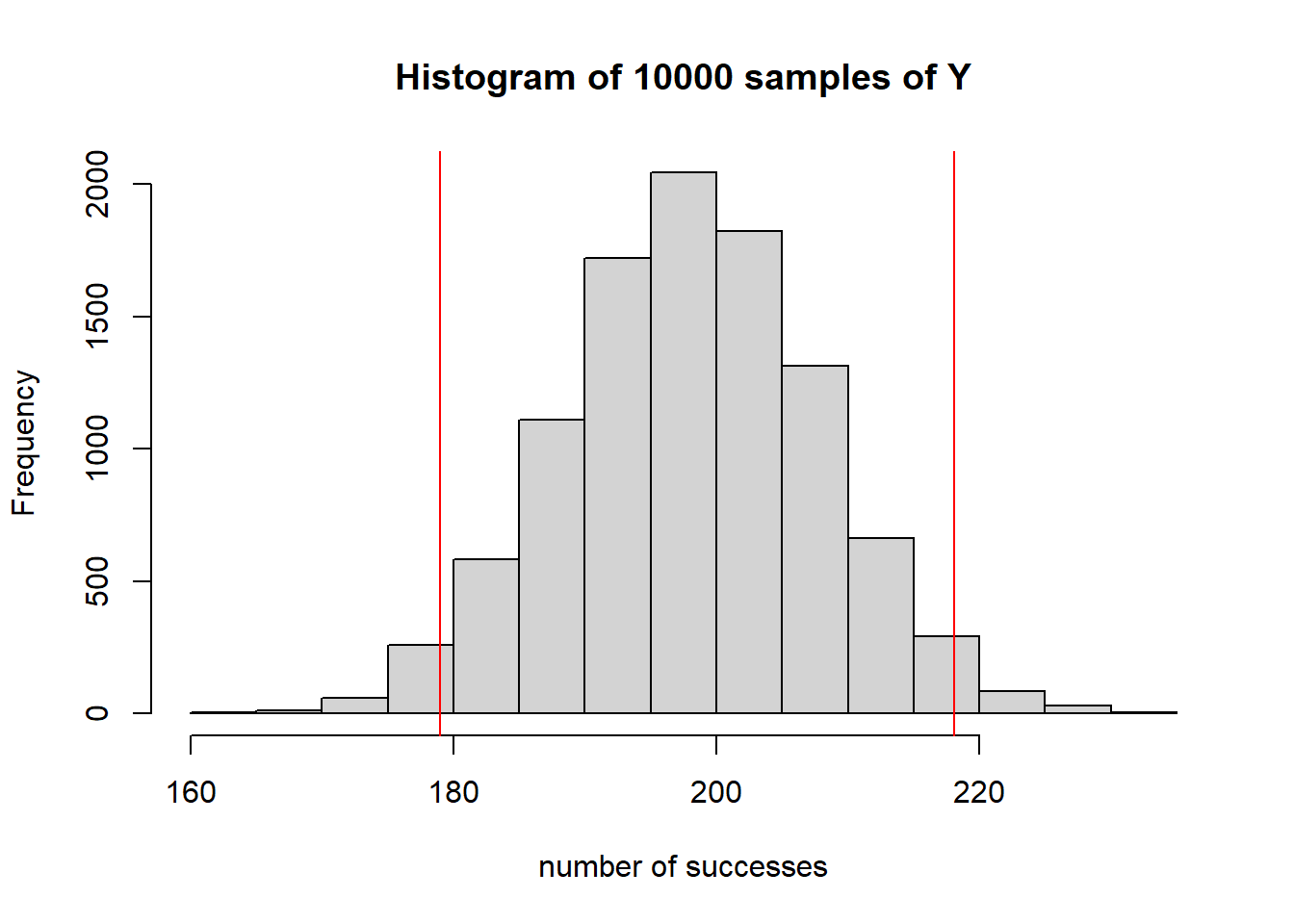
Now, when we think about the standard deviation here, it means the spread of the possible responses (successes) we might see. For a binomial distribution we know this to be \(\sigma = \sqrt {np(1-p)}\) which in this case \(\sigma = \sqrt{(384*0.517*(1-0.517))} = 9.79\). Further, because this data has a nice Normal shape, it’s fairly easy to interpret the standard deviation as the spread of this data, in terms of the number of successes we might see. The red vertical lines indicate the approximate 95% middle interval.
However, this is \(Y\), but instead we are more interested in \(\hat p\). A better illustration here would be to plot the distribution of \(\hat p\), which we can find by simply dividing by \(n\).
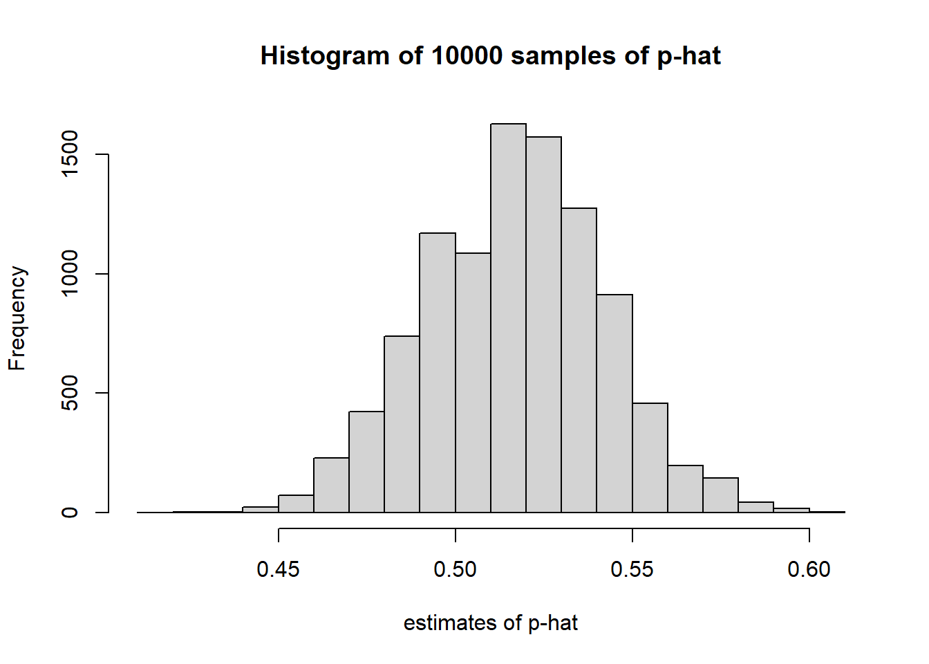
Note the main difference here is that the x-axis has changed.
Now, how much variation exists in this second distribution?
Here, we’ll calculate the standard error as \(SE_{\hat p} = \sqrt {\frac{p(1-p)}{n}} = \sqrt{(0.518*(1-0.518)/384)}\), which in this case is \(SE = 0.0255\).
Just to show this is meaningful, let’s add the \(\mu\pm2*SE\) values to our histogram.
lower <- mean(Y/384)-2*sqrt(0.518*(1-0.518)/384)
upper <- mean(Y/384)+2*sqrt(0.518*(1-0.518)/384)

hist(Y/384, xlab="estimates of p-hat")
abline(v=lower, col="red")
abline(v=upper, col="red")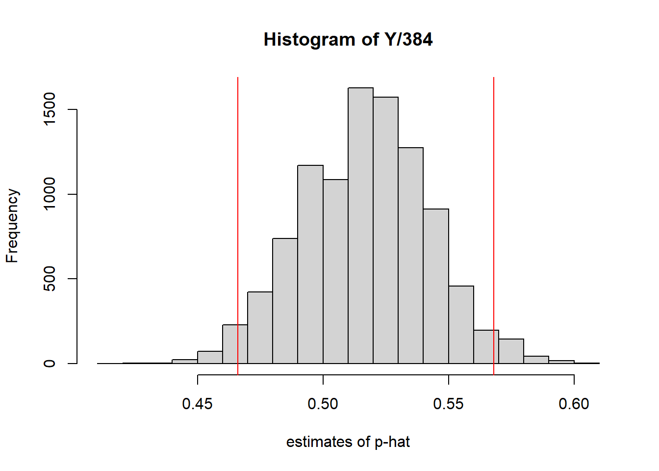
which hopefully illustrates that the middle 95% of the data lie within roughly 2 SE (standard errors) of \(\hat p\).
Quite simply, the standard error is an estimate of the spread of the data when we’re discussing (calculating) estimates of the mean parameter of the distribution, in this case \(p\).
The standard error is analogous to the standard deviation, but the difference is it refers to the uncertainty in the mean.
In fact, if we calculate the standard deviation of our simulated estimates of \(\hat p\), we see this gives basically the same results as the standard error formula does.
For our simulated data we find:
## [1] 0.02527703and based on the formula we find: \[SE = \sqrt {\frac{p(1-p)}{n}} = \sqrt{(0.517*0.483/384)} = 0.0255\]
In summary, when taking many samples from a population:
- the standard deviation describes the spread of the number of successes we’d see, whereas
- the standard error describes the spread of the estimates of \(\hat p\).
11.3.7 Optional: Deriving the Standard Error for the Binomial Distribution
Where does the equation for standard error come from? We can derive this pretty easily.
First, there’s a useful identity about variance of random variables. Let \(X\) be a random variable with a known variance \(Var(X)\). Consider the variable \(aX\) where \(a\) is some constant. Our identity says that the \(Var(aX) = a^2*Var(X)\). This makes some sense given our definition of variance from chapter 2.
So now, if we let \(Y\) be a random variable from a Binomial distribution with parameters \(n\) and \(p\), we know that \(Var(Y) = np(1-p)\).
Let \(\hat p = \frac{Y}{n}\) as we’ve defined above and we want to calculate the variance of \(\hat p\). Using our identity, we can find \(Var(\hat p) = \frac{1}{n^2}*Var(Y)\).
Substituting the value for \(Var(Y)\) we find \(Var(\hat p) = \frac{1}{n^2} * np(1-p) = \frac{p(1-p)}{n}\). Thus, the standard deviation of \(\hat p\) is \(\sqrt{\frac{p(1-p)}{n}}\), and to avoid confusion, we’re going to call this the standard error.
11.3.8 Standard Error and Sample Size
Of importance here, notice that \(n\) is in the denominator. What does this suggest as \(n\) gets large? What happens to our standard error?
.
.
.
.
What it means is that as \(n\) gets large, our standard error decreases, and therefore \(\hat p\) gets closer and closer to the true value of \(p\). Said differently, the more samples we take, the better our estimate of \(p\) is, which should be intuitive.
If I ask only 10 people who they’ll vote for (even assuming it’s not biased) that’s a horrible representation of \(p\). Alternatively, if I ask 10,000 people, that’s probably a pretty good representation of \(p\), assuming of course that my sampling is random. In the latter case our standard error will be much smaller.
11.3.9 Distributions vs Inference
By now you may be starting to think that we’ve been doing this wrong all along. If we never know \(p\), how do we use the binomial distribution?
The answer is we can get pretty close to \(p\).
As you saw with your histograms, they are Normally shaped. And based on the CLT, we can approximate the distribution of \(\hat p\) as being Normal.
With a bit of hand waving, we’re going to flip this slightly and say the true distribution of \(p \sim N(\hat p, SE_{\hat p})\), where
- \(\hat p= \frac{Y}{n}\) is our (one) sample estimate, and
- \(SE_{\hat p} = \sqrt {\frac{\hat p(1-\hat p)}{n}}\)
Here’s the exciting part about this: We can now create a confidence interval on where the true value of \(p\) lies.
Note: This formulation is technically incorrect because \(p\) is NOT a random variable, but instead a fixed value. So, it doesn’t come from a Normal distribution, in fact it doesn’t have a distribution at all! You should recognize that, and understand that this trick works fine only when thinking about confidence intervals as we will define them shortly.
11.3.10 Calculating Confidence Intervals
WARNING: The definition of a confidence interval is a bit confusing. Before I explain exactly what it means, let’s talk about how to calculate it.
Generally what we want is a reasonable estimate of where the true value of \(p\) lies. We know \(\hat p\) has a Normal distribution (as given above) and based on our knowledge of Normal distributions, we could calculate the interval where the middle 95% probability lies.
For example, if we know \(p \sim N(\hat p, SE_{\hat p})\) then our 95% interval is (\(\hat p -1.96*SE_{\hat p}\), \(\hat p +1.96*SE_{\hat p}\)). (Does anybody remember why is it 1.96?) Note that you would get the same result if you used qnorm() to find the 2.5% and 97.5% values.
This isn’t new. It’s the same as we previously calculated the middle 95% of the distribution.
11.3.11 Guided Practice
You are told \(p \sim N(0.52, 0.05)\), then what would the 95% CI (confidence interval) be?
11.3.12 Understanding Confidence Intervals
But what does this interval tell us in particular? Choose 1 of the following:
“95% of the intervals created this way will contain the true mean”
vs.
“There is a 95% chance the true mean lies within this interval”
Maybe its a technicality, AND I’m not sure it changes how you use it, but I think it’s important you understand the difference.
The following code displays 20 different 95% confidence intervals each created from a different sample from pop. The true value of \(p\) is given by the red line.
- How many of the confidence intervals contain the true value?
- How many (out of 20) would we expect to?
n <- 384
trials <- 20
plot(0,0, xlim=c(0.35, 0.70), ylim=c(1,trials), type="n", ylab="trial", xlab="confidence interval")
for (j in 1:trials) {
  a <- sum(sample(pop, size=n))/n
  se <- sqrt(a*(1-a)/n)
  points(a-1.96*se, j)
  points(a+1.96*se, j)
  segments(a-1.96*se, j, a+1.96*se, j)
}
abline(v=p, col="red")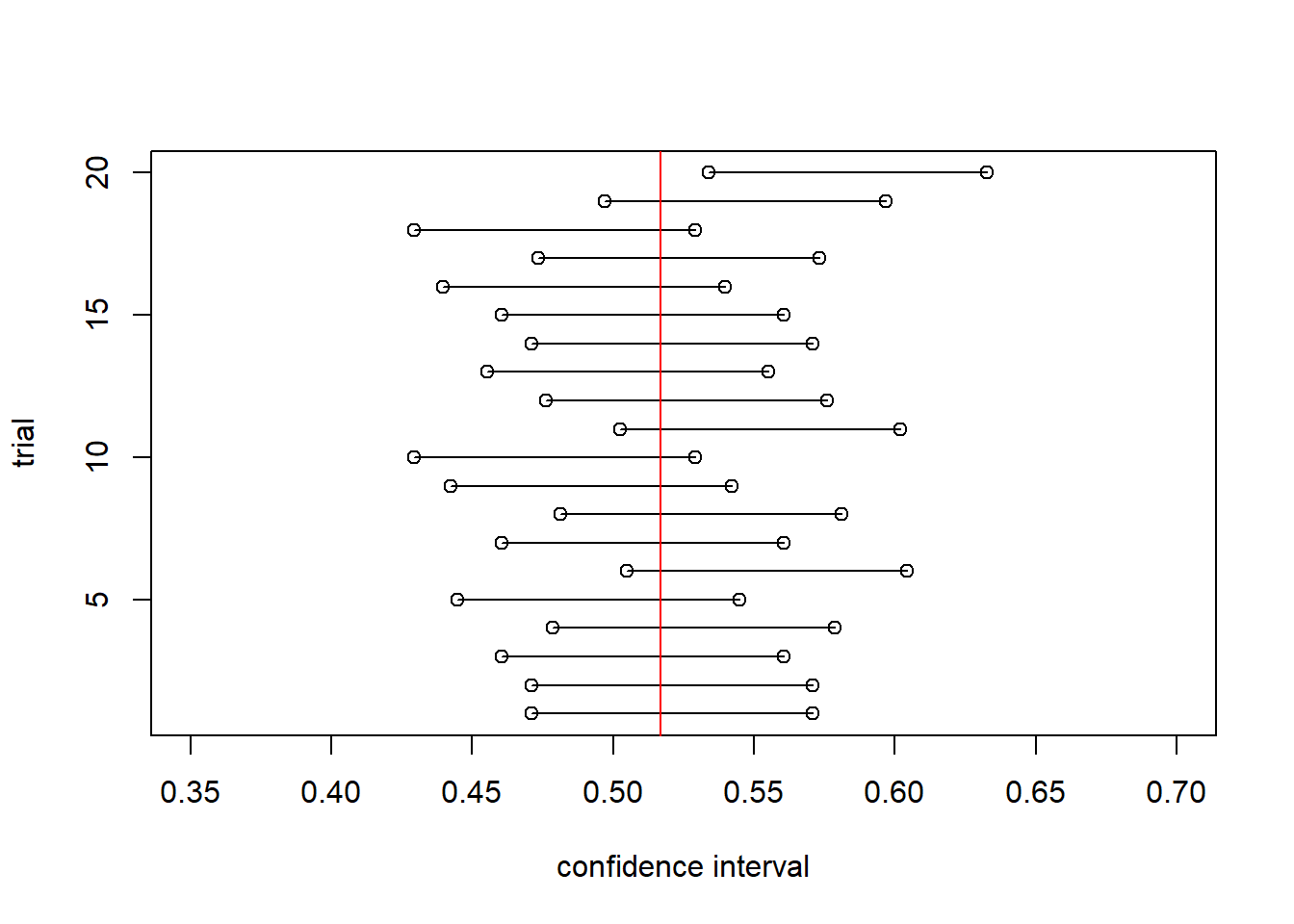
Hence, the correct answer is:
“95% of the intervals created this way will contain the true mean”
That is how we will define and interpret what a confidence interval means.
11.3.13 Notes on Using Standard Error for Inference on \(p\)
As discussed, we know the distribution of \(\hat p\) is \(N(p, SE_p)\). We could easily show that \(E[\hat p] = E[\frac{Y}{n}] = \frac{np}{n}= p\), and as we derived above, its standard deviation is \(SE_p\). Based on the CLT, a Binomial random variable quickly converges to Normal.
Of note, what we really desire is to make inference about \(p\), the true population value. Importantly, \(p\) is not a random variable, it is a constant (i.e. fixed), but unknown value.
Putting that aside for a moment, when we write a confidence interval on \(p\), we act as if \(p \sim N(\hat p, SE_{\hat p})\). Since \(p\) is fixed, this is NOT technically valid. If that equation were true, then we could say there’s a 95% chance that \(p\) is within the interval defined by \(\hat p \pm 1.96*SE_{\hat p}\). The reason we can make this leap (even though that equation isn’t true) has to do with likelihood calculations that are beyond the scope of this class. However, it because of this leap that we need to be careful when we’re interpreting what confidence intervals mean.
Since \(p\) is fixed, the inference we make is that “95% of the confidence created using this equation/approach will contain the true mean, \(p\).”
11.3.14 Guided Practice
According to a 2018 poll of \(n=1114\) people from Yale, (https://climatecommunication.yale.edu/about/projects/global-warmings-six-americas/) 59% of the survey respondents were either ‘Alarmed’ or ‘Concerned’ about climate change.
What is a 95% confidence interval on the true value of the percentage of people in America that are either ‘Alarmed’ or ‘Concerned’ about climate change?
11.3.15 Margin of Error
As a last topic of this section, often times you’ll see polling data that gives a result and a margin of error. What does that mean?
For example, before the 2020 election, a poll showed Joe Biden was leading Donald Trump 48% to 42% with a margin of error of 2.4%.
So, what does ‘margin of error’ mean? And how should we interpret it?
Quite simply, the margin of error (typically) is the distance from the mean (\(\hat p\)) to the edge of the 95% confidence interval. Or alternatively 1/2 the width of the confidence interval.
So, if we assume \(p=0.5\), and remembering that \(SE_{\hat p} = \sqrt {\frac{p(1-p)}{n}}\), the half width of the 95% confidence interval is \(1.96*SE_{\hat p}\). So, if \(n=384\) (as we used above), the margin of error is \(1.96*\sqrt{0.25/384} = 0.0500\), and hence a 5% margin of error. (In fact, that’s why I chose \(n=384\) above, because of the associated margin of error.)
More generally, we can calculate the Margin of error (or half-width of the 95% confidence interval) for different sample sizes, \(n\) as:
| \(n\) | Margin of Error |
|---|---|
| 384 | 0.05 |
| 600 | 0.04 |
| 1067 | 0.03 |
| 2401 | 0.02 |
If you’re interested in learning even more, see additional details here: * https://www.pewresearch.org/fact-tank/2016/09/08/understanding-the-margin-of-error-in-election-polls/
So, back to our original question, how do we interpret it? Based on our understanding of confidence intervals, we can say:
- the 95% confidence interval for Joe Biden’s support is between (45.6 and 50.4), and
- that the true value of Joe Biden’s support will fall in 95% of the confidence intervals we create this way.
We also then typically infer, looking at the above values, and in particular that Biden’s estimated \(p\) is outside of Trump’s estimated \(p\), that there is most likely a real difference between support for Biden and Trump.
We’ll see how to test this more explicitly in the next section.
11.3.16 Review of Learning Objectives
So, you should now be able to:
- Calculate \(\hat p\) from our sample, which will be our best estimate of the true population parameter, \(p\)
- Understand what standard error means and how to calculate it. Explain how standard error and standard deviation are different from one another.
- Create a confidence interval for proportion data, and explain what it means
- Describe what a “margin of error” is and how it relates to confidence intervals for polling data
11.4 Hypothesis Testing for Proportions
In the previous section we looked polling type data (binomial distribution) and learned about how to make inference for where the true value of \(p\) lies, based on our estimate of \(\hat p\) and \(n\).
In this section we’ll discuss how to do a statistical test to determine if the true value of \(p\) is different than our pre-sampling estimate. For example, maybe our hypothesis before sampling is that there isn’t a strong preference between two candidates or choices one way or the other, which would then suggest a hypothesized value of \(p = 0.5\) (i.e. equal support for both).
Based on assuming this (null) hypothesis is true, we will learn how to test whether our observed (sampled) results are reasonable.
Why would we want to do this?
This is a fundamental goal of statistics:
If we can determine (or conclude) that something is different than random, then there must be some underlying process. In other words, if it is NOT random, we have found something interesting!
11.4.1 Is the Difference Significant or Random?
(Trigger Warning - what follows is a difficult subject.)
The Mapping Police Violence group has created a database (https://mappingpoliceviolence.org/) that records police killings in the U.S. A good introduction to their work is given in this TED talk: https://www.ted.com/talks/samuel_sinyangwe_mapping_police_violence.
Diving into this, let’s suppose the percentage of people of color in a certain city is 28%. Let’s also suppose that of all the recorded police shootings, 35% of those were of people of color. Based on this, we might ask: Is that difference in percentage random or is there some underlying process causing people of color to more likely be involved?
Framing this slightly differently, our population here is the people in the city (and the percent that are POC), and our sample is those who were involved in police shootings.
We can use a statistical hypothesis test to determine this, building on the skills we’ve learned so far this year.
11.4.2 Learning Objectives
By the end of this section you should be able to:
- Explain the difference between a null and alternative hypothesis
- Describe how the “\(\alpha\)-level” impacts our test and state the standard value
- Calculate the test statistic for one sample tests of proportions
- Name and parameterize our null distribution, and explain what the null distribution represents
- Find the critical values of the null distribution based on \(\alpha\), and describe what those represent
- Calculate the p-value of our test and use it to either reject or fail to reject our \(H_0\)
- Determine how likely our observed results are under the null distribution, including using both the critical values and p-value
Note that these general steps will be the same process used across all of our hypothesis testing.
11.4.3 An example
The easiest way to explain this process is to simply do an example. Then we’ll come back through and clarify the terms and steps.
Switching to a lighter topic, let’s suppose we’re interested to understand if EPS students have a strong preference between Snapchat and Instagram. We’ll call preferring Snapchat a “success” and preferring Instagram a “failure”. (No judgment here.) We’ll also assume we’re randomly sampling so that we can assume our data are IID.
To start, we need to select a “Null Hypothesis”. (Note: I haven’t specifically defined Null and Alternative hypothesis yet, so briefly, you can think about these as our two options. Either null or alternative hypothesis must be true. We’re going to run a statistical test to decide which one is most likely.)
Our null hypothesis, which we denote \(H_0\), will be that there is NOT a strong preference between Snapchat and Instagram, and therefore results will be random, suggesting \(p=0.5\). (This is \(p\), our population parameter.) Our alternative hypothesis, \(H_A\) will then be that \(p\) is in fact statistically different from 0.5.
Next, we think about what the likely results of \(\hat p\) will be if \(H_0\) is true, namely if \(p=0.05\). Of course, from the previous section, you will realize this distribution will depend on \(n\), so let’s assume we plan to survey \(n=40\) students.
From the previous section, we also know something about calculating the error. In particular: \(SE_{\hat p} = \sqrt {\frac{p(1-p)}{n}}\). In this case, we use our null hypothesis value of \(p\) and find:
\[SE_{\hat p} = \sqrt{(0.5*0.5/40)} = 0.079\]
Why am I using \(p\) from our null hypothesis here, not \(\hat p\)? Because I want to know the distribution of \(\hat p\), i.e. the distribution IF the null hypothesis is true.
And thus we know from the CLT that \(\hat p\) will have a normal distribution and thus we can write our null distribution as \(\hat p \sim N(0.5, 0.079)\). Importantly: This is the distribution of values we’d expect to see for \(\hat p\) if the null distribution were true. The variation exists as a result of sampling variability. (This is what we previously simulated.)
Here is the plot of the null distribution:
p <- seq(from=0.25, to=0.75, by=0.01)
plot(p, dnorm(p, 0.5, 0.079), type="l", xlab="p", ylab="probability")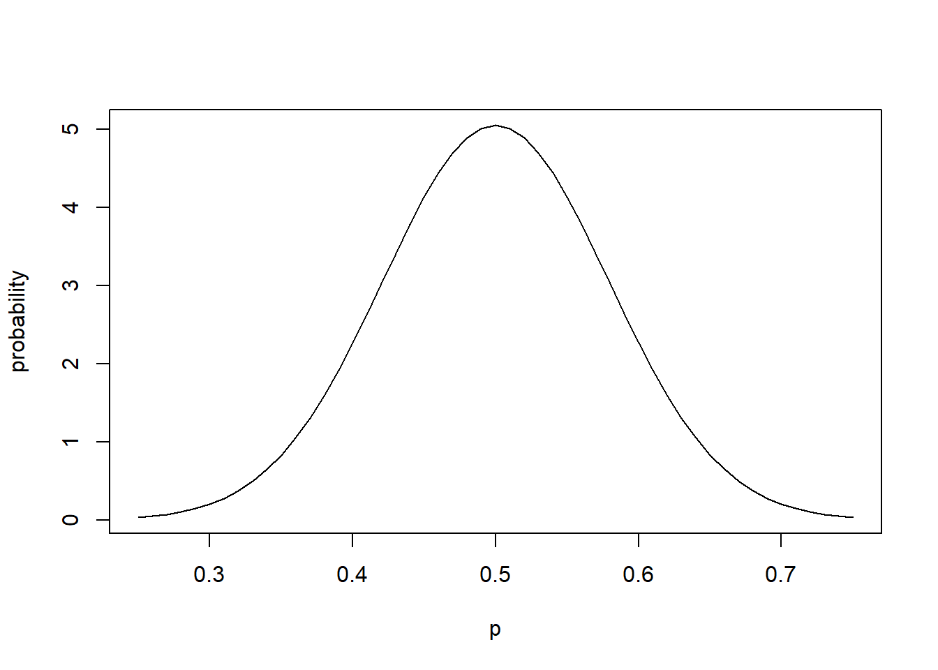
Lastly, we also need to decide on our so called “significance level” of the test, which we typically do by setting \(\alpha = 0.05\) With this, we are basically saying we’ll reject \(H_0\) if there’s less than a 1/20 chance that our sample data could have occurred randomly under \(H_0\). Think about how this might relate to the above plot, and more on this shortly.
Now we are ready to conduct our actual poll: we ask 40 students about their social media preference.
Suppose out of our 40 students, we find that 27 prefer Snapchat.
What is our “best estimate” of \(p\) at this point? Maybe its obvious, but since we had 27 successes out of 40 trials, we’ll set \(\hat p = \frac{27}{40} = 0.675\). This is our test statistic and we’ll use it in just a minute.
(Note: a big part of statistical inference has to do with figuring out what the best estimator of the population value is. Here we’re using what’s known as the “maximum likelihood estimator”.)
This value of \(\hat p\) itself is interesting, but isn’t (yet) enough to test \(H_0\). Why? We need to think about how likely this value is IF the null hypothesis is true. In other words, it depends on how much error is associated with that estimate.
Now our question is:
How likely would we be to see a value as extreme as 0.675 (our test statistic) if the null hypothesis is true (or I might say “under the null hypothesis” or “based on the null distribution”)?
Examine the following plot:
p <- seq(from=0.25, to=0.75, by=0.01)
plot(p, dnorm(p, 0.5, 0.079), type="l", xlab="p", ylab="probability")
abline(v=0.675, col="red")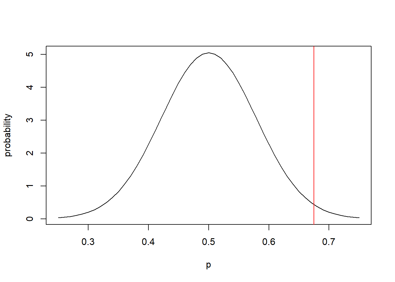
Here, the curve represents our null distribution on the likely values of \(\hat p\) if \(p=0.5\) given \(n=40\). The red line is the observed value of \(\hat p = 0.675\) based on our sample. So, how likely is the red value if the null hypothesis is true? And what does this suggest about whether \(H_0\) is true?
To solve this, we might think we could use pnorm(). But I need to be a little bit careful with respect to my \(H_0\). I’ve set this up as what’s called a two-tailed test. That means I would reject \(H_0\) if its too big OR too small, so I need to put 2.5% of the probability at each tail.
One approach is to use qnorm() to find the critical values that demarcate where I would reject \(H_0\). Note the critical values are those values of \(\hat p\), such that if our test statistic falls outside of which, I will reject \(H_0\), and if our test statistic falls inside of which, I don’t.
## [1] 0.3451628## [1] 0.6548372Let me redraw our distribution here, adding the critical values in green:
p <- seq(from=0.25, to=0.75, by=0.01)
plot(p, dnorm(p, 0.5, 0.079), type="l", xlab="p", ylab="probability")
abline(v=0.675, col="red")
abline(v=qnorm(0.025, 0.5, 0.079), col="forest green")
abline(v=qnorm(0.975, 0.5, 0.079), col="forest green")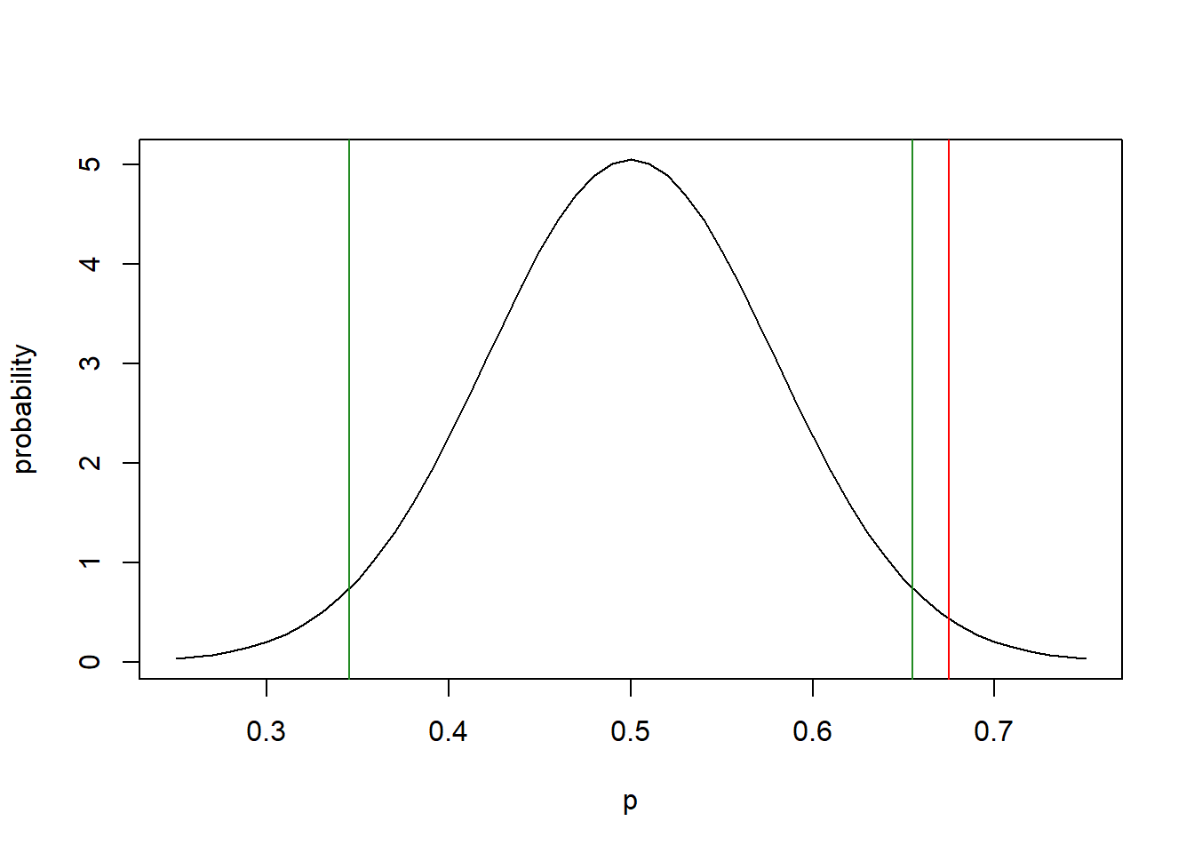
Now finally, we compare our test statistic of 0.675 to the critical values above and since our test statistic is larger than the upper critical value, we reject \(H_0\) in favor of \(H_A\) and hence conclude that there is a statistically significant difference between the true value of \(p\) and 0.5.
We’re done! Sort of…
There’s one more step that we usually do, namely to determine the p-value of the test statistic. The p-value represents “how likely is it to see a test statistic as extreme as ours (or more extreme) if the null hypothesis is true”. (and when I say extreme, what I’m really saying is… “as far away from the mean as …”)
Now let’s do that pnorm() calculation from above, and since we know the value is above the mean, let’s look at the upper tail probability. We find:
## [1] 0.01337352Since this is a two-tailed test, the p-value is twice (to account for both tails) the pnorm() result. So here, our p-value would be
## [1] 0.02674703This value means there is only about a 2.67% chance of seeing a value as extreme as \(\hat p= 0.675\) if the null hypothesis is true.
And since \(p=0.0267 < 0.05\) (remember we set our \(\alpha=0.05\)) we similarly conclude that we should reject \(H_0\).
Why use p-values? In addition to simply rejecting \(H_0\) (or not) we might also want to know the strength of the evidence. That’s what the p-value gives us in a standardized form.
Now we are done. It may seem that there were A LOT of steps involved, but you will quickly become comfortable with the process.
11.4.4 Hints on Calculating p-values
When calculating a p-value, we use the pnorm() function, but how do we know whether to use lower.tail=F or not?
The answer is: it depends on whether our test statistics (\(\hat p\) in this case) is below or above the mean of the distribution (\(p\) from \(H_0\) in this case.)
The following plot again shows our distribution and critical values.
x <- seq(from=0.25, to=0.75, by=0.01)
y <- dnorm(x, 0.5, 0.079)
plot(x,y, type="l", xlab="p-hat", ylab="probability")
abline(v=qnorm(0.025, 0.5, 0.079), col="forest green")
abline(v=qnorm(0.975, 0.5, 0.079), col="forest green")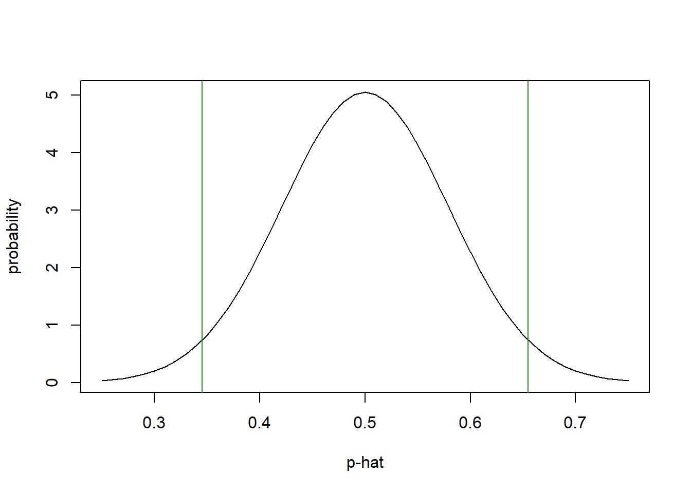
If \(\hat p\) is below the mean, such as say 0.30, we want the lower tail probability, so we’d use:
## [1] 0.01135287Alternatively, if \(\hat p\) is above the mean, such as say 0.65, we want the upper tail, so we’d use:
## [1] 0.05759944One critical note: p-values are probabilities, and as such must range between 0 and 1. If you ever find you’ve calculated a value bigger than that, check your work.
Also, in an unfortunate coincidence, p-values and \(p\) are NOT the same. This is often quick confusing.
11.4.5 Steps in the Hypothesis Testing Process
Overall, the process of hypothesis testing is to determine how likely our observed results are under the null distribution, and use this to probability to make conclusions about our initial hypothesis.
The following are the general steps we’ll use for all of upcoming hypothesis testing:
- Decide on our null and alternative hypothesis
- Determine our null distribution
- Pick our “alpha-level”
- Figure out our critical values
- Collect the data
- Calculate our “test statistic”
- Compare our test statistic to the critical values
- Calculate our p-value
- Reject or fail to reject \(H_0\) (if for example the p-value is less than \(\alpha = 0.05\))
11.4.6 Guided Practice
Based on the MPV (mapping police violence) dataset, in WA state there were 185 police shootings between 2013 and 2018. Of those, 23 were unknown race, 59 were PoC and 103 were ‘white’. If PoC comprise about 24% of WA state, is there a statistically significant difference between the percent in the population and the rate of being involved in police shootings ?
Make sure to work through all the steps of our hypothesis testing framework.
11.4.7 Review of Learning Objectives
By the end of this section you should be able to:
- Explain the difference between a null and alternative hypothesis
- Describe how the “\(\alpha\)-level” impacts our test and give the standard value
- Calculate the test statistic
- Name and parameterize our null distribution, and explain what the null distribution represents
- Find the critical values of the null distribution based on \(\alpha\), and describe what those represent
- Calculate the p-value of our test and use it to either reject or fail to reject our \(H_0\)
- Determine how likely our observed results are under the null distribution, including using both the critical values and p-value
And so now, combined with the previous section, you seen both statistical inference, which is concerned with understanding the likely values of a population parameter and hypothesis testing, which is a tool that allows us to evaluate if a population parameter could reasonably be a specific value, based on our sample data.
11.5 One-sided vs. Two-sided Tests
Suppose we’re interested to understand people’s views on whether they will take the COVID vaccine. However, instead of just testing if the population value is \(p=0.5\), we want to know if it’s greater than 0.7. In other words, does at least 70% of the population intend to take the vaccine once its available. Because of the inequality, this is an example of a “one-sided” test.
Note here that this is a slightly different situation that we evaluated previously. In particular, consider what value our test statistic would have that would lead us to what conclusion. And then, what type of the critical values would we need?
11.5.1 Learning Objectives
By the end of this section you should be able to:
- Explain the difference between a one-sided and two sided hypothesis test, including both why (and when) it is used, and how our execution of the test changes.
11.5.2 Running a One-sided Test
We’ll generally follow the same process here as we did with a two sided test. The two-sided test refers to the idea that we will reject \(H_0\) if our test statistic is too small OR too big. In other words, there are rejection regions on both sides of the distribution.
For a one sided test, we will only have one rejection region. Thinking back to our COVID vaccine example, we won’t reject if our test statistic is too big, only if it’s too small.
To start, let’s think about our null hypothesis. In this case, our null hypothesis is the not interesting idea that \(H_0: p<=0.7\). It’s generally the opposite of what we’re “hoping” to conclude.
As such, alternative hypothesis would be \(H_A: p>0.7\), because this would tell us that there is strong support for vaccinations, maybe enough to get to herd immunity.
Next, to parameterize our null distribution, note that this isn’t different than before. We still assume under \(H_0\) that it’s centered at 0.7 and we’ll calculate the standard error the same way we did previously. Assuming we poll 50 people, we’d find \(SE = \sqrt{0.7*0.3/50} = 0.065\).
So, under our specific \(H_0\), we calculate \(\hat p\sim N(0.7, 0.065)\).
Next, what is the critical value (singular) for our test at \(\alpha = 0.05\)?
Since we’re only doing a one-sided test, we’ll only reject if \(\hat p\) (our test statistic) is too large. We don’t care if it’s too small, that’s ok with our \(H_0\). And so our critical value is the point where ALL \(\alpha=0.05\) of the distribution lies above. In this case, we don’t split it in half.
x <- seq(from=0.5, to=0.9, by=0.01)
plot(x, dnorm(x, 0.7, 0.065), type="l", ylab="prob density")
a <- qnorm(0.95, 0.7, 0.065)
abline(v=a, col="red")
text(0.85, 2, labels = "5%", col="red")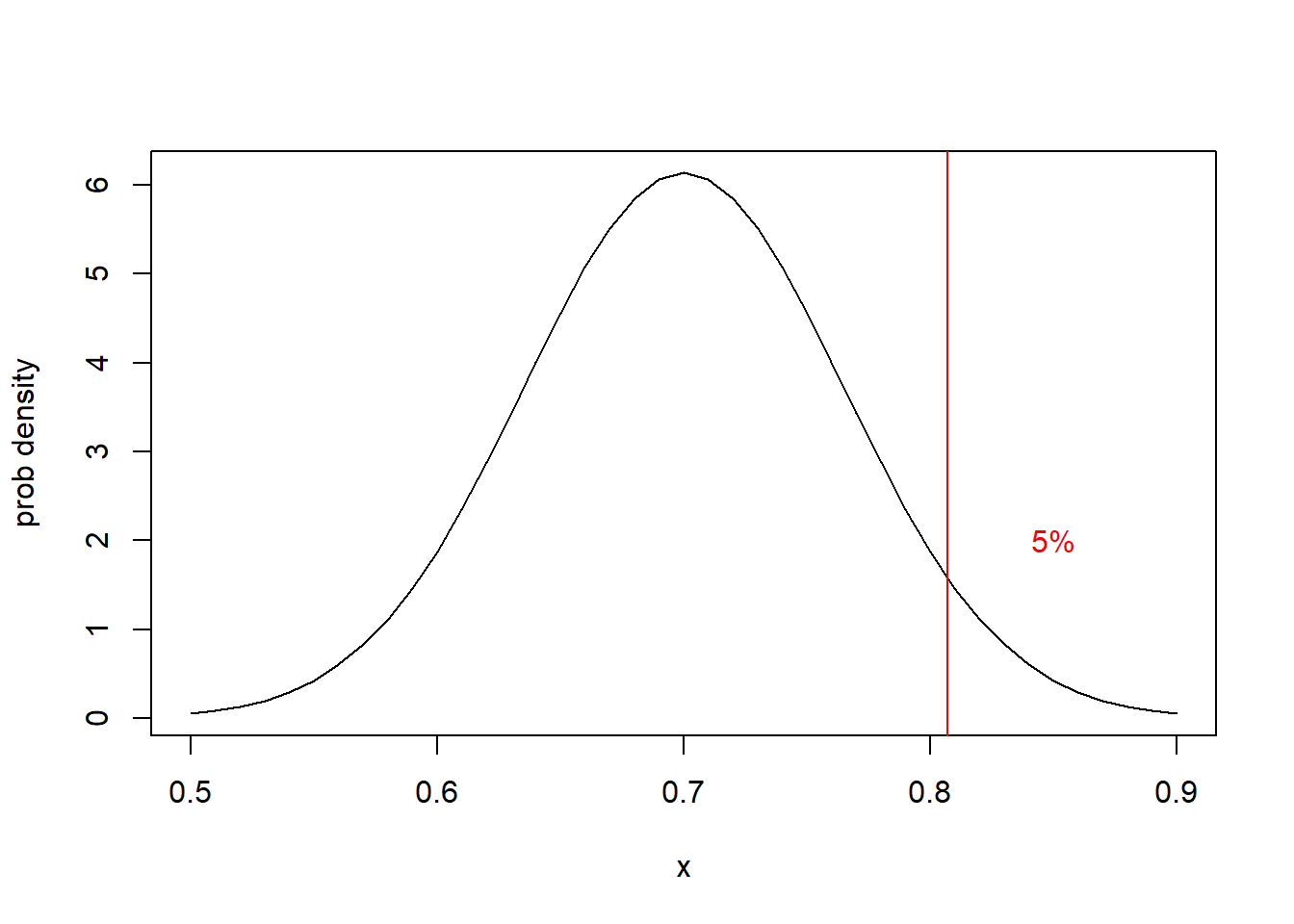
Of course we can find this critical value with:
## [1] 0.8069155So then you actually interview 50 people and find 31 say they intend to take the vaccine. What do you conclude?
We find our test statistic, \(\hat p\), is:
- \(\hat p = 37/50 = 0.74\)
Comparing this to our critical value (and note there’s only one in this case), we find \(\hat p\) < \(p_{crit}\) so we’d fail to reject \(H_0\) and conclude that there’s not enough evidence to reject the idea that true value of \(p\) may be 0.7 (even though our test statistic above below it).
Of course we may also want to find the actual p-value, namely the probability of seeing a test value as extreme as we did given \(H_0\) is true. Again this helps us understand the strength by which we ‘reject’ or ‘fail to reject’ \(H_0\).
For one sided tests, to determine the specific p-value of our test statistic, we only need to care about the tail we care about. In this case, and for our observed value:
## [1] 0.2691504which says there’s a 26.9% chance of seeing a value as extreme (low) as we did if the true value is \(p=0.7\). Again, based on our choice of \(\alpha = 0.05\), we’ll fail to reject \(H_0\) and conclude the true percentage of the people who intend to take the vaccine may well be below or at 0.7 (and that this higher observed value is thus just the result of random sampling.)
11.5.3 Where to Locate the Critical Value?
Why does it makes sense in this case to set \(H_A: p>0.7\) and subsequently use an upper tail critical value? Let’s think about the opposite situation. Suppose we had put the critical value below 0.7. In that case, a test statistic of \(\hat p=0.65\) would have been above the critical value and caused us to reject \(H_0\). But clearly 0.65<0.7 so we would be concluding \(p>0.7\) with scant evidence.
You also might think about two different questions here:
- Is it possible that \(p>0.7\)?
- Is it very likely that \(p>0.7\)?
In the first case you might want a lower tail critical value, whereas in the second case you definitely want an upper tail critical value.
The same logic applies when testing if an observed value is less than some predefined value.
11.5.4 Notes on One-sided Tests
- The approach for calculating a confidence interval doesn’t change. Meaning we still can use \(\hat p \pm 1.96*SE\) to calculate the likely range for \(p\).
- The big changes in hypothesis testing approach for one sided tests are:
- The null and alternative hypothesis are written differently
- There is only one critical value
- The p-value calculation is different
11.5.5 Guided Practice
For a one-sided test with \(H_0: p<=0.5\) and \(n=120\), you interview 120 people and find 63 people as ‘success’. Follow the steps described above to conduct a one sided test of \(H_0\). What do you conclude and why?
11.5.6 Review of Learning Objectives
By the end of this section you should be able to:
- Explain the difference between a one-sided and two sided hypothesis test, including both why (and when) it is used, and how our execution of the test changes.
11.6 Inference and Hypothesis Testing for Continuous Data
Above we discussed inference and hypothesis for count (proportion) data, the most common type of discrete data. There are other models for discrete data, however, we won’t be covering those in this class. Instead now we will move to looking at inference and hypothesis testing for continuous data. Since we will be primarily looking at estimating the mean of the distribution, we can rely on the CLT and assume the distribution of the mean has a normal distribution.
In what follows, we will see that our process for inference and hypothesis testing for continuous data is quite similar to what we used above. I will be clear to point out where differences occur, which are mainly related to our nomenclature and our calculation of the standard error.
For now, we are going to assume that \(\sigma\), the population level standard deviation is known. However, since this isn’t usually the case, in the next chapter we will discuss methods that don’t require that condition.
11.6.1 Learing Objectives
By the end of this section you should be able to:
Define our best estimate of the true population mean, \(\mu\), and calculate a confidence interval on where the true value lies.
Run a one-sided or two sided hypothesis test on the true value of \(\mu\), assuming \(\sigma\) is known. Steps here include:
- Define a null and alternative hypothesis for testing of continuous data
- Name and parameterize our null distribution, and explain what the null distribution represents
- Find the critical values of the null distribution based on \(\alpha\), and describe what those represent
- Calculate the test statistic, \(\bar X\)
- Calculate the standard error of the mean
- Calculate the p-value of our test
- Determine how likely our observed results are under the null distribution, and use the above information to either reject or fail to reject our \(H_0\)
11.6.2 Inference for Normal Data with \(\sigma\) known
Let’s suppose we were interesting in evaluating heights of EPS students. We go out and collect some data from \(n=30\) students and for our sample we find \(\bar X =64.8\) inches. (Remember, \(\bar X\) is our sample mean. And on a technical note, \(\bar X = \frac{\sum X_i}{n}\) is the maximum likelihood estimator of \(\mu\).)
Based on this sample, what can we infer about the entire student population? (As a reminder, when we consider “statistical inference”, our goal is to estimate the range where the true population value lies.)
As an important aside, our first question here should be about how the data was collected. Was it truly random? If not, the inference will be biased. We will discuss this further in a later chapter.
Putting sampling issues aside for now, how can we create a confidence interval on this estimate?
Once again, we need to know something about the sampling distribution of the average. We could do another simulation to find this, however the results will basically be the same. Our sample mean \(\bar X\) will have the following normal distribution:
\[\bar X\sim N(\mu, SE_{\mu})\]
This requires that we are able to find the standard error of the mean. Similar to with proportion data, for normal data \[SE_{\mu} = \frac{\sigma}{\sqrt{n}}\]
This approach requires that we know \(\sigma\), the population level standard deviation, possibly through a previous study. For now, let’s assume \(\sigma = 3.61\).
Note again that \(n\) is in the denominator of our standard error, suggesting as the number of samples increases, the error in our estimate decreases.
Using this information, for our sample we find \(SE_{\mu} = \frac{3.61}{\sqrt{30}} = 0.659\).
Therefore, \(\bar X \sim N(\mu, 0.659)\). And remember, to find our confidence intervals we “flip” this and act as if \(\mu\) is the random variable.
Hence, to find a 95% confidence interval on \(\mu\), we’ll use \({\mu-1.96*SE_{\mu}, \mu+1.96*SE_{\mu}} = {63.51, 66.09}\). Again, this means that 95% of the confidence intervals created this way will contain the true mean, \(\mu\).
So, it’s likely that the true mean \(\mu\) of student heights falls within the interval between \(63.51\) and \(66.09\) inches.
In summary, the only major difference here is how we calculate the value of the standard error.
11.6.3 Hypothesis Testing for Normal Data with \(\sigma\) known
What if we also (or instead) wanted to test our data against a specific value of \(\mu\)?
Again, let’s suppose we were interesting in evaluating heights of EPS students, however this time we have a prior idea that average height is 69.3 inches. Maybe, for example, we got this based on an estimate from another school or from a statewide average. So, our null hypothesis will be that the average height of EPS students is 69.3 inches and we want to test this hypothesis. Our alternate hypothesis is that \(\mu \ne 69.3\).
First, we should ask: Is this a one sided or two sided test?
Just for variety, here we’ll use slightly different data than we did above. In this case, we collect data from \(n=25\) students and find \(\bar X =65.2\). Is this difference (i.e. between \(\mu\) and \(\bar X\)) statistically significant? How would we know?
Remember our hypothesis testing steps (which are the same from before):
- Develop null and alternative hypothesis and determine our “alpha-level”
- Figure out and parameterize our null distribution
- Determine the critical values at the chosen \(\alpha\)
- Collect the data
- Calculate our “test-statistic”
- Figure out how likely our observed results are under the null distribution, including comparing the test statistic to the critical values and calculating the p-value
- Reject or fail to reject \(H_0\) (if for example the p-value is less than \(\alpha = 0.05\))
Formally we’ll write our null and alternative hypothesis as \(H_0: \mu = 69.3\) and \(H_A: \mu \ne 69.3\). The null hypothesis is typically our case where “nothing interesting is happening”. EPS heights are not different than the statewide average.
Next let’s construct our null distribution. For this data, with \(n=25\) and assuming \(\sigma=3.61\), we find \(SE_{\mu} = \frac{3.61}{\sqrt{25}} = 0.722\). We are sampling slightly fewer people than in our previous example which, means we have a slightly larger standard error.
From here our null distribution on \(\bar X\) is simply \(\bar X \sim N(\mu, SE_{\mu}) = N(69.3, 0.722)\). And note that we can determine this without collecting data, as long as we know what \(n\) is.
Why do we use 0.722 as our standard error here instead of 3.61? Ask yourself: “Are we thinking about the height of a random individual from the population or the calculated sample mean from a group of individuals?” Since it’s the latter, we’ll use the standard error NOT the standard deviation.
We can also calculate our critical values (for \(\alpha=0.05\)) assuming at two-sided test as:
## [1] 67.88491## [1] 70.71509Again, for a two sided test at \(\alpha=0.05\), we’re putting 2.5% of the distribution below the lower critical value and 2.5% of the distribution above the upper critical value.
Given this setup, what is the probability of seeing a value as extreme as our test statistic, \(\bar X = 65.2\), if the null hypothesis is true?
11.6.4 Draw The Picture!
Here is a plot of the null distribution (in black), the critical values (in blue) and the test statistic (in red).
x <- seq(from = 64, to =73, by=0.1)
plot(x, dnorm(x, 69.3, 0.722), type="l", ylab="probability")
abline(v=67.885, col="blue")
abline(v=70.715, col="blue")
abline(v=65.2, col="red")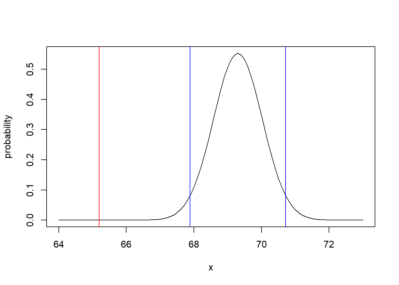
Just by inspection it seems very unlikely that our observed value of \(\bar X=65.2\) came from that distribution. And we see the observed value (red) is way outside of the critical values (blue).
To be complete, we can calculate the actual p-value as
## [1] 1.357458e-08which shows the probability is basically zero, and confirms what we saw in our sketch. Note: for our p-value in this case we’d probably write it as \(p<0.0001\) or similar.
Note: If you are confused by what 1.357458e-08 means, this is scientific notation and is equivalent to \(1.357\times 10^{-8}\), and so a very, very small number.
So, we would reject the null hypothesis and conclude there is a statistically significant difference between heights at EPS and the statewide average. (Make sure you always include the context of the problem when you write your conclusions.)
11.6.5 Guided Practice
An inventor has created a new type of lithium battery for laptops that is supposed to last longer. Existing batteries of this type have a life of \(\mu = 6.5\) hours with a population standard deviation of \(\sigma= 0.35\) hrs. A survey of 30 ‘new’ batteries had a mean \(\bar X = 6.75\) hours.
- Create a 90% confidence interval on the true value of the mean. (What multiplier do you need to use here?)
- Do a hypothesis test to evaluate if there is a statistically significant difference between the old and new batteries at \(\alpha=0.05\). Make sure to follow all the steps.
11.6.6 Review of Learning Objectives
Define our best estimate of the true population mean, \(\mu\), and calculate a confidence interval on where the true value lies.
Run a one-sided or two sided hypothesis test on the true value of \(\mu\), assuming \(\sigma\) is known. Steps here include:
- Define a null and alternative hypothesis for testing of continuous data
- Name and parameterize our null distribution, and explain what the null distribution represents
- Find the critical values of the null distribution based on \(\alpha\), and describe what those represent
- Calculate the test statistic, \(\bar X\)
- Calculate the standard error of the mean
- Calculate the p-value of our test
- Determine how likely our observed results are under the null distribution, and use the above information to either reject or fail to reject our \(H_0\)
11.7 Summary and Review
The following table compares our approach for creating confidence intervals on our parameter of interest using either proportion data or continuous data:
| item | Confidence Interval for proportion data | Confidence Interval for continuous data |
|---|---|---|
| population parameter | \(p\) | \(\mu\) |
| SE | \(\sqrt{\frac{\hat p*(1-\hat p)}{n}}\) | \(\frac{\sigma}{\sqrt{n}}\) where \(\sigma\) is the population standard deviation |
| 95% CI | \(\hat p \pm 1.96* SE\) | \(\bar X \pm 1.96*SE\) |
And remember that 95% of the confidence intervals created this way will contain the true value.
.
.
.
The following table compares our approach for hypothesis testing using either proportion data or continuous data:
| item | Hypothesis testing for proportion data | Hypothesis testing for continuous data |
|---|---|---|
| question | is \(\hat p\) from a distribution with mean \(p=p_0\)? | is \(\bar X\) from a distribution with mean \(\mu=\mu_0\)? |
| Null and Alternative | \(H_0: p = p_0\) , \(H_A:p \ne p_0\) | \(H_0: \mu = \mu_0\), \(H_A: \mu \ne \mu_0\) |
| SE | \(\sqrt{\frac{p*(1-p)}{n}}\) | \(\frac{\sigma}{\sqrt{n}}\) where \(\sigma\) is the population standard deviation |
| test statistic | \(\hat p = \frac{Y}{n}\) | \(\bar X= \frac{\sum x_i}{n}\) |
| Null distribution | \(\hat p \sim N(p,SE)\) | \(\bar X\sim N(\mu,SE)\) |
| critical values (at \(\alpha = 0.05\)) | \(p\pm 1.96*SE\) | \(\mu\pm 1.96*SE\) |
| p-values | pnorm(\(\hat p\), \(p\), SE) |
pnorm(\(\bar X\), \(\mu\), SE) |
where \(p_0\) and \(\mu_0\) are known values.
11.8 Exercises
Exercise 11.1 You take a random survey of \(n=75\) people from a larger population and find \(\hat p = 0.613\).
- How many successes did you see?
- What is the standard error?
- What is the distribution of \(\hat p\)? Name the distribution and give its parameters.
- Calculate a 95% confidence interval on \(p\) using
qnorm()for the distribution of \(p\).
- Calculate a 95% confidence interval on \(p\) using \(\hat p +/- 1.96* SE\).
- Prove to yourself that your answers to (c) and (d) are equivalent.
Exercise 11.2 You sample 500 people and find 275 people indicating they will likely vote for your candidate.
- What are \(n\) and \(Y\)? What is your estimate of \(\hat p\)?
- What is the standard error?
- What is the 95% confidence interval on \(p\)?
- What is the margin of error?
Exercise 11.3 A recent poll of \(n=1000\) people (https://thehill.com/hilltv/what-americas-thinking/412545-70-percent-of-americans-support-medicare-for-all-health-care) found that 42 percent of respondents said they “strongly” support a single payer (i.e. universal) health care system and 28 percent said they “somewhat” supported it.
- What is \(\hat p\) for this poll?
- What is \(SE_p\) for this poll?
- What is the margin of error on this poll?
- What is a 95% confidence interval on the true percentage of people in the population who somewhat or strongly support a single payer approach? How do you interpret this confidence interval?
- Based on this, how would you describe the evidence of support in the population for universal health care?
Exercise 11.4 Create a plot of the standard error for different values of \(p\), assuming \(n=250\).
- First create \(x\), a vector of p ranging from 0 to 1 with a step of 0.02.
- Then create \(y\), a vector of SE calculations based on \(x\) and \(n\).
- Plot \(x\) vs \(y\).
- What do you notice? For what value of \(p\) is the standard error the greatest? How much variation exists in the standard error, particular between \(0.35 < p < 0.65\)?
- What does your plot suggest about whether \(p\) or \(n\) is more important for understanding standard error?
Exercise 11.5 You take a sample and find \(\hat p=0.43\).
- What is the standard error if \(n = 600\)?
- What is the standard error if \(n = 1200\)? How do your answers to (a) and (b) compare?
- What is the 95% confidence interval on p if \(n=600\)?
- What is the 99% confidence interval on p if \(n=600\)? How do your answers to (c) and (d) compare?
Exercise 11.6 Assume that our sampling distribution of \(p\) is normal with a mean of \(\hat p =0.45\) with a standard error of \(SE=0.08\).
- Can you determine the sample size (\(n\))?
- What is the probability that the true value of \(p\) is above 0.5?
Exercise 11.7 Write a few sentences explaining the difference between the standard deviation and standard error.
Exercise 11.8 Write a few sentences explaining why the standard error decreases as the sample size increases.
Exercise 11.9 Write a few sentences explaining what a 95% confidence interval means.
Exercise 11.10 Write a few sentences explaining how the Central Limit Theorem is related to estimating the sampling distribution of \(\hat p\).
Exercise 11.11 Suppose we are interested to evaluate how EPS students feel about having a finals week during Fall and Winter trimesters. You interview \(n=45\) students and find 32 say they strongly support it.
- What is your \(H_0\) (null hypothesis)? What is your \(H_A\) (alternative hypothesis)? Make sure to write these in terms of \(p\).
- What is the null distribution based on your null hypothesis? What type of distribution is it and what are the parameters of the distribution?
- What are the lower and upper critical values at \(\alpha = 0.05\)?
- What is the value of your test statistic (i.e. your observed value of \(\hat p\))?
- What is the p-value associated with your test statistic?
- What do you conclude?
- How many people would have had to say “yes” for you to change your conclusion?
Exercise 11.12 Write a few sentences explaining the what a p-value is. Does a higher or smaller p-value give more evidence for rejecting \(H_0\)? Does it matter if our test statistic is above or below the mean?
Exercise 11.13 Write a few sentences explaining what the difference between using a p-value to make our conclusion is versus simply comparing our test statistic against our critical values. What does using a p-value tell us that the critical values do not? Is there ever a case where the two methods would yield different conclusions?
Exercise 11.14 Suppose you are interested to evaluate support for some type of tax in Puget Sound to help fund Orca recovery.
- How many people do you need to interview to have margin of error of 2.5%? (assume \(p=0.5\) for this calculation)
- What are your null \(H_0\) and alternative \(H_A\) hypothesis?
- What is your null distribution (including the type of distribution and the values of the associated parameters)?
- What are the critical values at \(\alpha = 0.05\)?
- Now suppose you interview the number of people calculated above (for your margin of error), and find 720 people in support, what is your \(\hat p\)?
- Based on \(\hat p\), what do you conclude about \(H_0\)?
- What is the p-value?
Exercise 11.15 What happens to your critical values as \(\alpha\) changes? For example imagine that \(\hat p \sim N(0.4, 0.025)\). Calculate the critical values at \(\alpha = 0.05\) and again at \(\alpha = 0.01\). What do you observe about the values. Does this make it easier or harder to reject \(H_0\)? Given what you know about \(\alpha\), why does this make sense?
11.8.1 One-sided vs. Two-sided testing
Exercise 11.16 You are interested in testing if an observed proportion is less than 0.51.
- What is your null hypothesis?
- If you sample 200 people, what is your critical value at \(\alpha=0.05\)?
- If you find a value of \(\hat p = 0.45\) what do you conclude?
Exercise 11.17 For a one-sided test with a null hypothesis of \(H_0: p \le 0.667\) and you interview 180 people and find 123 people as ‘success’. Follow the steps described above to conduct a one sided test of \(H_0\). Be explicit about your alternative hypothesis, critical value(s), test statistic and p-value.
- What do you conclude and why?
- How many people would have had to say “yes” for you to change your conclusion?
Exercise 11.18 Write a few sentences explaining the what happens to critical values in one sided vs. two-sided tests?
Exercise 11.19 What happens in a one sided test if the observed test statistic is extreme, but in the opposite direction? For example if we are testing \(H_0 < 0.5\) and find a test statistic that is very small?
11.8.2 Hypothesis Testing with \(\sigma\) Known
Exercise 11.20 Assume carbon emissions in the US per person are Normally distributed with a mean of \(\mu = 18\) mton per person with a standard deviation of \(\sigma = 1.8\) mton per person. You wonder if people in the PNW (Pacific Northwest) are consistent with this estimate given that much of our electricity is generated from hydropower and given general attitudes in the PNW. You randomly survey \(n=25\) people and find a sample mean, \(\bar x=16.5\) mton per person. For this analysis, use the population standard deviation.
- What is the standard error of your estimate?
- What is a 95% confidence interval on your estimate of the mean of people in the PNW?
- Is it reasonable to assume that people in the PNW are the same as the rest of the country or not? Run a hypothesis test at \(\alpha=0.05\), detail your null distribution, calculate your test statistic and determine the p-value. What do you conclude?
Exercise 11.21 The following data shows a sample of social media usage by EPS students (in hrs/wk). Assume the national average for this age group is 5.5 hrs/day with a standard deviation of 1.33 hrs/day. Run a hypothesis test (at \(\alpha = 0.1\)) to evaluate if EPS students use social media more than the average. What do you conclude?
smu <- c(7.28, 5.84, 5.11, 5.24, 4.94, 7.01, 4.17, 8.02, 4.88, 4.83, 5.40, 6.55, 7.87, 7.39, 5.51, 4.29, 5.10, 7.38)
Exercise 11.22 Assume your null distribution for \(\bar X\) is \(N(12.8, 2.1)\).
- Sketch the null distribution using R.
- Assuming a two-sided test at \(\alpha=0.05\), add the critical values to your plot as vertical lines.
- If your test statistic is \(\bar X=16.8\), what do you conclude? What is the associated p-value?
- Now assume a one-sided test with \(H_0: \mu \le 12.8\) at \(\alpha=0.05\), add the critical value to your plot.
- Using the same test statistic as part (c), now what do you conclude? What is the associated p-value?
- Given that both (b) and (d) are \(\alpha=0.05\) tests, explain why your conclusions are different.
Exercise 11.23 Write a few sentences explaining the relationship between p-values, \(\alpha\) and critical values?
Exercise 11.24 Write a few sentences explaining the how our ability to reject a difference between \(\bar x\) and \(\mu\) changes as \(\sigma\) gets bigger.