Chapter 4 Introduction to Probability
4.1 Overview
In this chapter we will be discussing probability, and in particular work to understand and quantify concepts of random processes and outcomes. We will define probability rules and learn how to manipulate those rules using Algebra. We will look at the intersection and union of different events, whether independent or not, and what any such interaction might mean. Finally we will introduce the use simulation to experiment with different types of sampling from various populations. (A lot of those terms are probably new - don’t worry! We’re just at the overview.)
4.1.1 Understanding Risk (the game)
How many of you have played Risk, the game of global domination?
In the game, you start with a certain number of armies and you’re trying to take over the world. You battle other players in adjacent territories by rolling dice based on the number armies you each have. Ties go to the defender. Here’s an example battle:
Attacker (rolls 3 dice):
## [1] 4 5 1Defender (rolls 2 dice):
## [1] 6 1In this case the attacker and defender would each lose 1 army.
This is an example of using a discrete uniform distribution where the results are independent of one another. Further, we can calculate explicitly the probability that the attacker wins for various scenarios (#’s of armies).
At a higher level, understanding probability and probability distributions is fundamental to understanding statistics, so that’s where we’ll start. And analyzing games hopefully makes it fun! We’ll come back to analyzing games shortly.
4.1.2 Learning Objectives
By the end of this chapter you should be able to:
- Define basic probability terms: probability, random variable, event, outcome, independence, disjoint, mutually exclusive, complement
- Write the relationship between events outcomes and probabilities using probability notation
- Apply logical operations OR and AND and calculate associated probabilities for simple combinations of outcomes
- Distinguish between events that are disjoint or not, and events that are independent or not
- Apply the ‘addition’ and ‘multiplication’ rules for probability and explain how the assumption of independence can be used to simplify both rules
- Define what joint and marginal probabilities are and explain where joint and marginal probabilities appear in 2x2 (or similar) contingency tables
- Calculate both joint and marginal probabilities given the appropriate information
- Demonstrate how to evaluate whether multiple events appear to exhibit independence
- Create and use a contingency table based on probabilities or counts, including converting between counts and probabilities (or proportions). Calculate and fill in missing values. Interpret the various cells.
Additionally, using R you should be able to
- Simulate discrete random data using the
sample()function, including creating the full set using theseq()andc()functions - Differentiate between sampling with and without replacement
- Define and plot what a probability distribution is
- Understand how simulation can help illustrate the “Law of Large Numbers”
4.1.3 Why does randomness exist?
Does randomness really exist in the world? This is a fascinating question that is probably beyond the scope of this class, but here are some resources you might explore:
- Galton Board (http://mathworld.wolfram.com/GaltonBoard.html)
- The Not so Random Coin Toss (https://www.npr.org/templates/story/story.php?storyId=1697475)
- Schrödinger’s cat: A thought experiment in quantum mechanics (https://www.youtube.com/watch?v=UjaAxUO6-Uw)
- What is the Heisenberg Uncertainty Principle? (https://www.youtube.com/watch?v=TQKELOE9eY4)
We will take the approach that randomness does exist, either because of its inherent role in the nature of the universe and/or in cases where deterministic causes are unknowable.
4.2 Probability, Random Processes and Outcomes
4.2.1 What are Random Processes?
Let’s think about flipping a coin, drawing a card or rolling dice. Those are all events, where the actual result is not known before hand. For our purposes, an event is something that happens (or will happen) and has more than one possible results or outcomes. For example if our event is flipping a coin, then the possible outcomes are Heads or Tails. Or if an event is rolling two six sided die, then the outcomes might be the possible values of the sum of those two dice, namely the values 2 through 12.
There is a random aspect to the outcomes. We don’t know the result before the event occurs. We also might distinguish between possible outcomes (i.e. before) and actual outcomes. Again, the random process leads to an outcome. For actual outcomes, we might see a Head (for the coin flip), or a sum of 8 (for rolling two dice).
Before the event occurs, we don’t know the outcome, but we may know the probability of each possible outcome. The probability of an outcome is the proportion of times the outcome would occur if we observed the random process an infinite number of times. We can often calculate the probability explicitly, based on assumptions of fairness. Probabilities range between 0 and 1 (or 0 and 100%). The sum of the probabilities of all outcomes for an event equals 1, since one of the outcomes is sure to happen.
For example, a fair die can take values of 1, 2, 3, 4, 5 or 6, each with equal probability. Since there are six (6) different outcomes that are all equally likely, each outcome has a probability of 1/6th. However, the outcomes of the sum of two dice (the values between 2 and 12) do NOT occur with equal probability.
4.2.2 A bit about Notation
To assist our notation, we will often use letters \(A\), \(B\), etc. to denote a particular event, particularly in the case where that event is binary, i.e. it either occurs or not. So we might define the event A to be drawing a red 2 from a fair deck of cards and then write \(P(A) = 1/26\), where the \(P()\) operator stands for “the probability of”. There are 2 red cards in the deck and 52 cards total. We’ll also use the exclamation point to denote that A didn’t happen, e.g. \(P(!A) = 25/26\).
Additionally, for events with multiple outcomes, we will often define a random variable, such as \(X\), as a placeholder for the unknown outcome. For example, if our event was rolling a six-sided die, \(X\) would be the unknown value of the die. We don’t know what value \(X\) takes until after we roll. Importantly, before the event occurs we can write \(P(X = 3) = 1/6\), or in words " the probability of rolling a three is 1/6th".
4.2.3 Set Notation of Probability
This brings up a more general result that, in the case where each outcome is equally likely:
\[P = \frac{S}{n}\]
Where \(S\) is the number of outcomes we consider a “success” and \(n\) is the total number of outcomes.
For example, in the case of rolling an odd number on a 8 sided die, there are \(n=8\) total outcomes, but only \(S=4\) of those are “successes” (an odd number) and so the probability of rolling an odd = 4/8 = 1/2.
Note that if the probability of each outcome is NOT equally likely, we need a more complicated approach, which we will cover in subsequent chapters.
4.2.4 Guided Practice
For each of the following, define the event, suggest a random variable, list the possible outcomes, and if possible calculate the probabilities of each event.
- Drawing a card from a 52 card deck
- Drawing a spade from a 52 card deck
- Flipping a coin 4 times
- Rolling two six-sided dice
- The number of electoral votes won by the D candidate
(and note, there may be multiple answers to each of these.)
4.2.5 Observed vs. Theoretical Probabilites
Does this mean that exactly 1/6th of our rolls will be fours? Let’s try it. Take a die and roll it 40 times and record your results (you can work in pairs or groups). If you don’t have a die available, use the following R code to simulate a single roll:
## [1] 1First write down a table as follows. Have one person roll the die and the other tally the results.
| Value | # of times |
|---|---|
| 1 | |
| 2 | |
| 3 | |
| 4 | |
| 5 | |
| 6 |
Next, calculate the proportion of occurrences. For example, if I rolled the dice 40 times and saw eight (8) 5’s then my proportion is 8/40 = 1/5 = 0.20.
We will use \(\hat p\) (“p hat”) to denote the observed probability (as calculated or estimated) and use \(p\) for the true probability.
In statistics, we often take a (small) sample to get an estimate AND we’ll use that estimate to make inference about the population, the true value. (Wait, is there always true value? Let’s come back to that later.) So in this case, you are using your rolls to estimate \(\hat p\) values, whereas we expect \(p =1/6\).
Q: What did everyone get?
I’ll put your results into an R object and calculate the mean. You can follow along if you’d like. Then I’ll plot a histogram and we can talk about the variation that occurred.
Q: What does this tell you about fairness?
Q: Why was there variation? What does the histogram show?
Again, what was \(X\) (our random variable) here? What is our outcome? And what do your proportions add to? Why?
In general, this question about true probabilities versus sample probabilities will occupy much of time later in the course. For now, we’ll continue on with understanding the mathematical rules of probability, which are applicable in either case.
4.3 Probability Rules
Now, with that overview of probability, outcomes and random variables under our belt, let’s dive deeper into the mathematics. This section will contain a list of probability rules that we need to learn.
Definition 4.1 (Sum of Multiple Outcomes) If an event \(A\) has \(n\) outcomes, and we notate \(A_i\) as outcome \(i\), \(P(A_1) + P(A_2) + ... + P(A_n) = 1\).
Definition 4.2 (Complement Rule) If an event \(A\) has only two outcomes (e.g. H or T), then \(P(A) + P(!A) = 1\) where \(!A\) indicates that A doesn’t happen and is read as “not A”.
Definition 4.3 (Addition Rule (for Disjoint Events)) If two events \(A\) and \(B\) are disjoint (or mutually exclusive), meaning they cannot simultaneously happen, then the probability that one or the other happens is \(P(A\ or\ B) = P(A) + P(B)\).
Definition 4.4 (Multiplication Rule for Independence) For two events \(A\) and \(B\) that are independent of one another (meaning they don’t affect each others outcomes) the probability that both happens is \(P(A\ and\ B) = P(A) * P(B)\).
Definition 4.5 (General Addition Rule) For any two events \(A\) and \(B\) the probability that one or the other happens is \(P(A\ or\ B) = P(A) + P(B) - P(A\ and\ B)\).
Definition 4.6 (Joint Probabilities) For any two events \(A\) and \(B\), the marginal probability of one is the sum of its joint probabilities, or \(P(A) = P(A\ and\ B) + P(A\ and\ !B)\).
In what follows we will discuss each of these rules in more detail.
4.3.1 The Sum of Probabilites for an Event Always Equals 1
Remember our definition of an event. Simply, it’s something that happens or not, an in particular something for which there is uncertainty. It could be:
- drawing an Ace
- rolling a 3
- getting into the college of your choice
- whether it rains tomorrow
All of those have uncertainty about them, and as written they are all binary.
Again, we’ll often use letters for random variables for events. So we might write if \(A\) is the event of drawing an Ace, then in probability notation we’d write this as \(P(A)\) and say this as the “probability of A”.
Probabilities must range between 0 and 1, where 0 means it will NOT happen and 1 means it absolutely will happen. \(P(A) = 0.5\) means there’s a 50% chance event A will happen.
And, if we add up the probabilities for all the possible outcomes for a given event, it must sum to exactly 1. If we enumerated ALL of the possible outcomes for an event, then one of those outcomes must occur.
Considering the card drawn from a deck, it could be a 2, 3, 4, … 10, J, Q, K, or A, of various suits. In this case, each out these outcomes are mutually exclusive (meaning only one result can happen.) And, since one of those must happen we know: \[P(2) + P(3) + P(4) + ... +P(10)+P(J)+P(Q)+P(K) + P(A) = 1\]
4.3.2 NOT and Complement
A simple example of the above rule is seen when looking at an event that only has two outcomes. For example, if \(P(A)\) is the probability of rolling a 3, then \(P(!A)\) is the probability that we don’t roll a 3. The exclamation sign indicates NOT and is read the “probability of NOT A”.
Then, we can talk about the complement rule, which says:
\[P(A) + P(!A) = 1\]
This simply restates the point that the probability of all outcomes must sum to 1 (or 100%).
It can then easily be shown (via subtraction) that
\[P(!A) = 1 - P(A)\]
For example, suppose that there are three choices for lunch which you get at random: pasta, sandwich or salad. If probability of getting a salad is 0.25, what is the prob of not getting a salad? \(P(!salad) = 0.75\)
Additionally, you should recognize that we can manipulate the above probability rules using standard algebra.
4.3.3 Definition of logical OR and AND
We now turn our attention to looking at multiple events, and we’ll start again with some definitions. Given 2 events, A and B:
Definition 4.7 (AND) \(A\ and\ B\): means that both A and B happen simultaneously. For example I could draw a card that is both a 5 and red (heart or diamond). But I can’t draw a 5 and a 2 at the same time, assuming I draw only one card. In mathematical notation, AND is the same as intersection \(A \cap B\).
Definition 4.8 (OR) \(A\ or\ B\): means that A or B or possibly both occur. For example, I could ask about drawing a 3 OR a 4 from a deck of cards, which notably can’t both happen. I could also ask about drawing a 3 OR a black card, which then includes the possibility of drawing a black 3. Both of those are OR calculations. In mathematical notation, OR is the same as union, \(A \cup B\).
4.3.4 Disjoint (or Mutually Exclusive) Events and the Addition Rule
If we roll a six sided die, we might ask:
- what is the probability of rolling a 2 or 4?
- what is the probability of rolling a value less than five (1, 2, 3, or 4)?
As discussed above, assuming a fair die, the probability of rolling any individual number 1 through 6 equals 1/6. Intuitively, the the probability of rolling a 2 or 4 is 1/3. The probability of rolling a value less than five (1, 2, 3, or 4) is 4/6 = 2/3.
However, it’s worth proving out intuition with math. To figure out the probability of any one of a set of events occurring, we’ll take advantage of the idea that rolling each numbers is mutually exclusive (also known as disjoint).
Definition 4.9 (Mutually Exclusive) Two events A and B are mutually exclusive if they cannot occur simultaneously. Also known as disjoint. For example, a single roll of a die only has one outcome. The event of rolling a 2 and the event of rolling a 3, cannot both happen simultaneously if only rolling a single die. Similarly, you can’t flip a H and T on the same coin toss.
We can explicitly quantify this for mutually exclusive (disjoint) events using the Addition Rule, which says that \[P(A\ or\ B) = P(A) + P(B)\] Read this as “the probability of events \(A\) or \(B\)”. Since the events here are disjoint, OR means simply one or the other.
So using this equation, to find the \(P(2\ or\ 4)\), we have \(P(2\ or\ 4) = P(2)+P(4) = 1/6+1/6 = 1/3\), matching our intuition above.
In our second example we see that we can easily extend this rule to handle more than two events.
Again, this rule is only applicable if the events are disjoint, meaning they can’t happen at the same time. Are the following events disjoint?
- wearing white socks or blue socks
- wearing white socks or a green shirt
- going to an Ivy League school and having a successful life?
We’ll see a more general rule that relaxes this assumption shortly.
4.3.5 Guided Practice
- For a single die roll of an 8 sided dice, what is \(P(3, 4, 5,\ or\ 6)\)?
- For a single die roll of an 8 sided dice, what about \(P(1, 2, 3, 4, 5\ or\ 6)\)?
- For a 52 card deck, what is the probability of drawing a face card?
- For a single die roll, what is \(P(1, 2, 3,\ or\ 4)\) OR \(P(2, 4,\ or\ 6)\)?
- Come up with examples from your life of events that are mutually exclusive and events that are not.
4.3.6 Independence, Joint Probabilities and the Multiplication Rule
Now let’s talk about logical AND, and to do that we’ll introduce a second die. (Of course, for disjoint events, which cannot happen simultaneously, the probability of both A and B is always 0.)
What’s the probability that when rolling 2 six sided dice, that we roll 2 fours? Said differently, what’s the probability that die 1 = 4 AND die 2 = 4? To calculate this we need to discuss the idea of independence.
Definition 4.10 (Independence) Independence between events A and B means that the outcome of one event does not influence the outcome of the other event.
Assuming a fair die, the probability of the first die being a four is independent of the probability of the second die being a four. In other words, the probability that first die is a four (if we knew that in advance) wouldn’t give us any more information about whether the second die will be a four. It doesn’t make it more or less likely. The outcomes are independent of one another. They don’t affect each other.
If events are independent, then we can multiply their probabilities to find their joint probability, i.e. \[P(A\ and\ B) = P(A)*P(B)\] So in this case, the \(P(4\ and\ 4) = 1/6 * 1/6 = 1/36\).
This is known as the Multiplication rule for independent processes. And it can be applied for more than two processes.
Let’s do an example. If we draw a single card from a fair 52 card deck, what is the probability that we draw a black face card?
First, is the probability of a card being black independent of the probability of that card being a face card? In other words, does the probability that a card is black (if we knew that) give us any more information about whether it is a face card? (Discuss)
.
.
.
.
In fact, yes, they are independent. There are the same number of face cards in each suit, so knowing the color doesn’t help us at all. Similarly, knowing the card is a face card doesn’t tell us its color.
So, what is the probability that we draw a black face card? Well, let’s break it down. Our two so-called marginal probabilities are \(Pr(black) = 26/52=1/2\) and \(Pr(face\ card) = 12/52 = 3/13\).
Then the probability that we draw a black face card is Pr(black) times Pr(face card) \(= \frac{1}{2} * \frac{3}{13} = \frac{3}{26}\). And note, there are exactly 6 black face cards in the deck, so these are equal and independence makes sense.
4.4 Joint and Marginal Probabilities under Independence
Previously we discussed the probability of randomly drawing a Spade and a face card. Since we are looking at two events happening together, this is known as the “joint” probability.
Taking a step back, each card has multiple attributes or characteristics, or variables for lack of a better word that are associated with it. Two are obvious: color and value.
And this is true for other things too. People can be R vs. D and drive an electric car or not. They can be under or over 21 and can use social media more or less than 10 hrs per week. Etc., etc.
So, back to our card example, what is the probability a randomly drawn card is a Diamond and 5 or below (including the Ace)? In particular it’s the AND here that indicates we’re calculating a joint probability. Similar to what we did previously, we can write this in a 2x2 table as:
| card | P(\(<=5\)) | P(\(>5\)) | Total |
|---|---|---|---|
| P(Diamond) | 0.25 | ||
| P(!Diamond) | 0.75 | ||
| Total | 0.384 | 0.616 |
where this table now contains the probabilities instead of the counts. The values on the far right column and bottom row (under Total) are known as the marginal probabilities. In this case (0.384, 0.616, 0.25 and 0.75).
Now you go ahead and attempt to fill out the rest of this table, assuming independence between card color and value.
To get you started, note that under the condition of independence, we know: \(P(A\ and\ B) = P(A)*P(B)\). You should be able to use this rule to find all four joint probabilities.
.
.
.
.
As a first example, \(P(Diamond\ and <=5) = P(Diamond)*P(<=5) = 0.25*0.384 = 0.096\). In fact there are 5 out of the 52 cards in the deck that meet this condition and \(5/52= 0.096\), confirming the result.
And, here is the complete table:
| card | P(\(<=5\)) | P(\(>5\)) | Total |
|---|---|---|---|
| P(diamond) | 0.096 | 0.154 | 0.25 |
| P(!diamond) | 0.288 | 0.462 | 0.75 |
| Total | 0.384 | 0.616 |
Interestingly, for any row or column, we find the sum equals its parts, such as: \(P(diamond) = P(diamond\ and\ <=5) + P(diamond\ and\ >5)\), right? Said differently, the marginal probability is the sum of the appropriate joint probabilities. (We’ll codify this rule shortly.)
4.4.1 Finding Joint and Marginal Probabilities
So now, let’s suppose I gave you the information the other way. If we are given a joint probability and one marginal probability, how would we find the other marginal probability?
For example, let’s look at event \(A\) as “do you play sports?” and event \(B\) as “do you live in Bellevue?” Assume these are independent.
If we know that the P(play sports and live in Bellevue) = 12% and the probability that you play sports is 40%, what is the probability you live in Bellevue? At first it may seem like we don’t have enough information to solve this, but in fact, we do!
Here’s the 2x2 table to start.
| P | play | don’t play | total |
|---|---|---|---|
| Bellevue | 0.12 | ||
| ! Bellevue | |||
| total | 0.40 |
Can you fill out the rest of this table? Yes, if you:
- rely on our assumption of independence,
- use our rule that \(P(A\ and\ B) = P(A)*P(B)\), and
- remember the complement rule.
.
.
.
.
My approach is to:
- First, arrange the multiplication rule as \(P(B) = P(A\ and\ B) /P(A)\), and using this allows me to know the \(P(Bellevue) = \frac{0.12}{0.4} = 0.3\).
- Next, we can calculate the missing marginal probabilities as, \(P(!A) = 1 - 0.4 = 0.6\), and \(P(!B) = 1 - 0.3 = 0.7\).
- Then, I can calculate any (and all) of the missing cells using the appropriate marginal probabilities. For example, \(P(A\ and\ !B) = P(A)*P(!B) = 0.7*0.4 = 0.28\).
- The rest of the table is similarly found as \(P(!A\ and\ B) = 0.6*0.3 = 0.18\) and \(P(!A\ and\ !B) = 0.6*0.7 = 0.42\)
| P | play | don’t play | total |
|---|---|---|---|
| Bellevue | 0.12 | 0.18 | 0.3 |
| ! Bellevue | 0.28 | 0.42 | 0.7 |
| total | 0.40 | 0.6 |
Of importance, note that the sum of all of the joint probabilities must equal 1 (since one of those combinations must happen.)
4.4.2 Guided Practice
Create a 2x2 table and determine both the joint and marginal probabilities if \(A\) is the event that a family at EPS owns an electric car and \(B\) is the event that they have more than one student at EPS. Let \(P(A) = 0.2\) and \(P(B) = 0.15\), and assume that these events are independent. Find the four joint probabilities and the two missing marginal probabilities.
Let’s look at the relationship between state population and gun ownership in the PNW (which I’ll define to include WA, OR, ID and MT). Of the overall population, the breakup by states is roughly: WA 52%, OR 29%, ID, 12%, MT 7%. So if we randomly sampled people in the PNW, there’s a 52% chance they’d be from WA. And, for the region as a whole, 67% don’t own guns and 33% own 1 or more gun.
- Suppose two people are selected at random. What is the probability that both are from WA? What is the probability that neither are from WA?
- Supposing state and gun ownership are independent, what is the probability that random person is from OR AND owns one or more guns?
- Supposing state and gun ownership are independent, what is the probability that random person is not from WA AND doesn’t own a gun?
| num of people | WA | OR | ID | MT | total |
|---|---|---|---|---|---|
| don’t own a gun | 0.67 | ||||
| own one or more gun | 0.33 | ||||
| total | 0.52 | 0.29 | 0.12 | 0.07 |
In other words, here I’ve given you the marginal probabilities, so can you fill out a table with the joint probabilities?
- What is the relationship between independence and joint probabilities? (Discuss)
4.4.3 Converting between Marginal and Joint Probabilities
We used this rule above, but didn’t discuss the algebra. Specifically it says that the marginal probability is the sum of the corresponding joint probabilities.
\[P(A) = P(A\ and\ B) + P(A\ and\ !B)\]
What does this say and why/when is it true? Does it depend on the assumption of independence?
Using the above example, the probability that I live in Bellevue is (i) the probability that I live in Bellevue AND I play sports + (ii) the probability that I live in Bellevue AND I don’t play sports.
4.4.4 Guided Practice
- For the following two events A and B, fill in the missing values, assuming independence. In this case, try to use the relationship between joint and marginal probabilities to fill in the missing cells.
| P | A | !A | total |
|---|---|---|---|
| B | 0.1 | ||
| !B | |||
| total | 0.35 |
- Can you prove that \(P(A) = P(A\ and\ B) + P(A\ and\ !B)\) is true? Hint: replace both joint probabilities with the multiplication rule for independence, then factor and use the complement rule.
4.4.5 OR Probabilities for Events that are not Disjoint
So far we’ve talked about how to calculate OR and AND probabilities if we have disjoint events. (Remember AND probabilities must =0 if disjoint!) We’ve also discussed how to calculate AND probabilities if we have independent events. Here we’ll discuss OR probabilities for events that are independent but NOT disjoint.
Q: Back to our deck of cards, what is the probability of drawing a Spade OR a drawing a face card? And, let’s think about why can’t simply we use our addition rule here.
To illustrate this situation, let’s put all 52 cards into a 2x2 table and let \(S\) be the event of whether we draw a Spade and \(F\) be the event of whether we draw a face card.
| card | \(S\) | \(!S\) |
|---|---|---|
| \(F\) | 3 | 9 |
| \(!F\) | 10 | 30 |
where again I’m using the !, i.e. NOT, to represent the complement.
We’ll use this 2x2 table approach often in this and the next chapter, particularly for describing the interaction between two events. Values within a 2x2 table can either be counts or probabilities. Here we are using counts. In the above table, the value of 3 represents the idea that 3 cards are both spade and face cards. 30 cards are neither spades or face cards.
What we see here is that some overlap exists in the probability of outcomes between our events. There are cards that are both Spades and face cards, illustrating why these events aren’t disjoint.
Using the above table, we can calculate:
- \(P(S) = \frac{3+10}{52} = \frac{1}{4}\) (the whole left column)
- \(P(F) = \frac{3+9}{52} = \frac{3}{13}\) (the whole top row)
- \(P(S\ and\ F) = \frac{3}{52}\) (the upper left cell)
When we think about our question, \(P(S\ or\ F)\), we want \(\frac{3+9+10}{52} = \frac{22}{52}\)
However, if we apply our standard addition rule, \(P(S) + P(F)\), we double count the group of cards which are both Spades and face cards.
To account for this, the General Addition Rule says that \[P(A\ or\ B) = P(A) + P(B) - P(A\ and\ B)\]
In our specific case we’d have \(P(A\ or\ B) = \frac{1}{4} + \frac{3}{13} - \frac{3}{52} = \frac{22}{52}\). Note that we subtract out the overlap.
Another way to think of this is we’re taking the top row and left column of the table, and we don’t want to count the upper left box twice.
(and note that if \(A\) and \(B\) are disjoint, then \(P(A\ and\ B) = 0\), so this general rule will simplify appropriately.)
4.4.6 Guided Practice
What is the probability of drawing a red card OR a card less than 5? Create the 2x2 table with all outcomes and confirm the general addition rule works.
Suppose that the probability of extreme drought is 12%, the probability of major wildfire smoke impacting air quality is 25%, and the probability of both is 20%. What is the probability that either experiencing either extreme drought or major wildfire smoke (or both)?
Explain what is meant by “overlap” and why we need to account for it.
4.4.7 OR and AND Probabilities for Events that are not Independent
As we defined above, if two events are not independent it means that they affect each other. Knowing one is true may make it more (or less) likely that the other is true. How would we find \(P(A\ and\ B)\) in this case? We would need to know much more about the relationship between \(A\) and \(B\) to figure this out. In this case, we can’t determine \(P(A\ and\ B)\) based on \(P(A)\) and \(P(B)\) alone.
However, if we are given \(P(A\ and\ B)\), then we can still use the general addition rule of the previous section for calculating OR probabilities. Importantly, that rule holds regardless of independence or not.
For AND probabilities however, we’re a bit stuck. What we can do is use the multiplication rule to evaluate the extent to which observed results exhibit independence.
For example, the following table shows the interaction between two events G and H.
| prob | G | !G |
|---|---|---|
| H | 0.1 | 0.3 |
| !H | 0.4 | 0.2 |
From this table we see \(P(G) = 0.5\) (summing the left column) and \(P(H) = 0.4\) (summing the top row). If these events were independent, we’d expect \(P(G\ and\ H) = 0.5*0.4 = 0.2\). However from the table we actually observe \(P(G\ and\ H) = 0.1\). Since these are not the same it means that events G and H are NOT independent.
4.4.8 Guided Practice
- For the following table of probabilities, are the events A and B independent? Why or why not?
| prob | A | !A |
|---|---|---|
| B | 0.21 | 0.32 |
| !B | 0.35 | 0.12 |
- What is the probability of drawing a single card this is both red and less than 5? Are these two events independent? Demonstrate that the multiplication rule is (or isn’t) applicable here.
4.5 Evaluating Joint Probabilities from Count Data
Let’s do another example looking at whether independence exists based on count data. A 2019 Pew Research poll asked people about their beliefs on a range of issues and their political leanings. What do you see?

Figure 4.1: Results from a Pew Research poll asking people about their beliefs on a range of issues and their political leanings.
What does this data show? In particular, do you think there’s independence between political affiliation and beliefs on different issues? Probably not, because for certain issues R’s show more concern whereas for other issues D’s express more concern. Hence concern appears to be dependent upon (and hence is NOT independent of) the specific issue.
In this section we’ll evaluate how to fill in and evaluate 2x2 contingency tables when the assumption of independence does NOT hold.
Let’s now assume 1307 Americans were specifically asked: “Is there solid evidence that the average temperature on Earth has been getting warmer over the past few decades?” as well as their party affiliation. (Modified from problem 3.15 in OpenIntro Stats)
A useful way to display the results is through a contingency table:
| /# | Earth is Warming | Not Warming | Total |
|---|---|---|---|
| Republican | 222 | 379 | 601 |
| Democrat | 562 | 144 | 706 |
| Total | 784 | 523 | 1307 |
What does this table show you? Can you calculate:
- The probability that a random person was a Republican?
- The probability that a random person believes the Earth is warming?
- Whether these are independent? (Probably not, right?)
In fact I’m not sure our brains are that good at looking at this and easily understanding it. So, let’s dive a little deeper, and look at the same data written as proportions.
4.5.1 Converting from Counts to Proportions
Here is the table from above as marginal and joint proportions, which we’ll manipulate similar to probabilities:
| P | Earth is Warming | Not Warming | Total |
|---|---|---|---|
| Republican | 0.17 | 0.29 | 0.46 |
| Democrat | 0.43 | 0.11 | 0.54 |
| Total | 0.60 | 0.40 | 1.00 |
First, how did I calculate these values? Note that 0.17 = 222/1307 and 0.46 = 601/1307, so in this case we’re dividing each observed count by the total number of responses. That’s the only way to make sure the joint probabilities sum to 1.
And so, here we’ll use observed proportions to represent probabilities under the assumption that the result are representative of our population.
Q: So, what does the value 0.11 represent?
.
.
.
.
It’s the the joint probability of someone being in the “Democrat AND Not Warming” group, and note that these probabilities refer to the whole group (the numbers in red). As we saw above, the whole probability distribution must add to 1 and here we see \(0.17+0.29+0.43+0.11 = 1\).
Now, what if we wanted to think about events A or B in isolation? The marginal probability of P(Earth is warming) = 0.60. This represents the overall probability of believing the Earth is warming for the whole group. In our table this is found by adding the two sub groups that believe the Earth is warming. (i.e. the blue numbers in the first column.) As a reminder, marginal probabilities occur both in columns and along rows.
Q: Does this mean that 43% of Democrats believe the Earth is warming?
No, it means that 43% of our whole sample fall in the bucket of both being Democrats AND believe the Earth is warming. Is this clear?
So to review, marginal probabilities are __________________ and joint probabilities are __________________.
Choose one:
- on the outside edge (typically right or bottom)
- in the center of the table
4.5.2 Notation for Joint and Marginal Probabilities
For the above table, to make our lives a little easier, let’s define:
- Let \(A\) be the event if a person is Republican, and so \(!A\) is if the person is Democrat
- Let \(B\) be the event if the person believes the Earth is warming, and hence \(!B\) is if the person does not believe the Earth is warming.
Q: If I write \(P(A) = P(A\ and\ B) + P(A\ and\ !B)\) how would you put that into words in this specific example?
Again, this is how we convert from joint to marginal probabilities.
- What is \(P(B)\) in this same format (i.e. as a function of joint probabilities)?
- What is \(P(!A)\) in this same format (i.e. as a function of joint probabilities)?
So in general, (even without the assumption of independence) we can convert between joint and marginal probabilities using this equation. In words we can say that the marginal probability is the sum of the associated joint probabilities. And again, this is true regardless of whether events A and B show independence.
Lastly, in the case where we have independence, we can also use our Multiplication Rule for Independence, namely \(P(A\ and\ B) = P(A)*P(B)\) to convert between marginal and joint probabilities.
4.5.3 Do Observed Probabilities Exhibit Independence?
Now let’s answer the question about whether the above data exhibit independence. If party affiliation and beliefs on global warming were independent, what counts would we expect?
| P | Earth is Warming | Not Warming | Total |
|---|---|---|---|
| Republican | 0.17 | 0.29 | 0.46 |
| Democrat | 0.43 | 0.11 | 0.54 |
| Total | 0.60 | 0.40 | 1.00 |
To evaluate this we can look at any of the cells and compare the observed proportions with the predicted proportions if independence were true.
For example, if we look at the cell which shows the proportion who are Republican and don’t believe in warming, we see a value of 0.29. If being a Republican were independent of beliefs about warming, then we would expect \(0.46*0.40 = 0.184\) proportion of the responses to fall in this cell.
This difference suggests that party affiliation and beliefs on global warming are NOT independent.
4.5.4 \(\chi^2\) GOF Testing
So I assume you’re all wondering, OK how would we really know independence about or not??? There must be a better way, right? That’s a little ahead of where we are (yet), but we’ll get there, probably in the second trimester. To summarize, we’ll look at how far away our data are from the expected result. And then evaluate how likely that is based on randomness alone. If the chance of seeing data that extreme assuming \(H_0\) is true, is less than 5%, we’ll reject our hypothesis of independence. I can say more, but we can also wait…
4.5.5 Guided Practice
- This following data comes from Stanford Open Policing Project (https://openpolicing.stanford.edu/) which we’ll do more with later in the year. Let’s imagine we have two events concerning people who are pulled over by the police. We’ll let event \(A\) be whether the person is white or not and event \(B\) be whether the person is subsequently searched.
| p | A | !A | total |
|---|---|---|---|
| B | 0.20 | ||
| !B | 0.35 | ||
| total | 0.55 |
- Use what you know about the relationship between marginal and joint probabilities to fill in the rest of the table, and make sure not to assume independence at this stage.
- Does the assumption of independence between race and subsequent search seem appropriate here?
- Let’s suppose we’re looking at social media use by age and take a random sample of 1000 people with cell phones in WA state. We categorize people between 13-25 and 26 and above (old people) and also ask how many hours per week they spend on their phones on social media (less than 10 or more than 10). Before looking at the data, would you expect age and hours on social media choice to be independent? Why or why not?
The data for this problem is shown below:
| age | P(\(<=10\) hrs) | P(\(>10\) hrs) | Total |
|---|---|---|---|
| P(13-25) | 102 | 448 | 550 |
| P(26+) | 198 | 252 | 450 |
| Total | 300 | 700 |
- Convert the above table to proportions.
- Does this table show independence? Why or why not?
- What is the probability that a random person is over 26 AND spends less than 10 hrs on social media per week?
- What is the probability that a random person is under 25 OR spends less than 10 hrs on social media per week?
4.6 Visualizing Probability Distributions
When discussing probabilities, it can be useful to visualize them, and so its worth introducing concept of Probability distributions. Previously we said that all possible outcomes for an event must sum to 1, i.e. P(\(A_1\)) + P(\(A_2\)) + … P(\(A_n\)) = 1. How could we visualize this?
We might represent our dice roll as follows:

This shows our possible outcomes on the x axis, ranging from 1 through 6, and the probability of each on the y-axis. You might think this looks like a histogram, and you’d be right!
So, to determine the probability of rolling a 1 or 2, just add the probability (read “heights”) of the appropriate bars. We will use the idea of going from distributions to probabilities a lot this year. In particular, this is what’s known as a discrete uniform distribution. The outcomes are discrete, and the associated probabilities are uniform, or all the same.
What would the probability distribution for the outcomes of the sum of two dice look like? (You’ll calculate the actual probabilities as part of your exercises. )
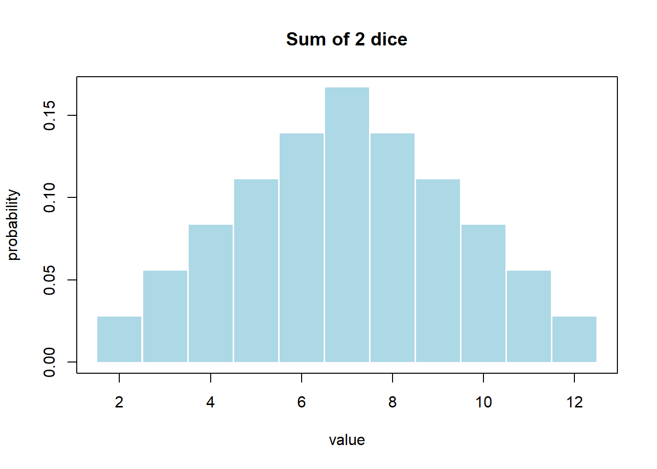
We’ll do a lot more with Probability Distributions later in this course but two main takeaways with probability distributions are that:
- they contain all possible outcomes
- the total distribution must sum to 1
4.7 Introduction to Simulating Discrete Random Variables
In this section, we will introduce the idea of how we can simulate a random variable. Above we discussed the idea of a random variable, here we will illustrate it.
4.7.1 Using the sample() function
The sample() function is the workhorse of discrete distributions in R.
Looking at it’s R help we see the usage is:
sample(x, size, replace=FALSE, prob=NULL)
where:
xis the vector from which to choosesizeis the number of items to choosereplaceis a Boolean variable indicating if sampling should occur with replacementprobis a vector of probability weights for obtaining the elements being sampled
We will work examples that illustrates the use of each of these parameters.
4.7.2 Rolling a 6-sided die
Here we will simulate how to roll a six sided die. With any call to the to sample we need to define the set of elements from which we will draw, and possibly the associated probabilities.
To simulate a 6-sided die, we want our set to be the integers 1 through 6. To create this, we use the seq() function as:
## [1] 1 2 3 4 5 6Hence, to simulate a single roll of a 6-sided die, we set size=1.
## [1] 3Every time this executes, this generates a random result. Try it!
4.7.3 Summing two dice
To simulate the sum of two dice, we follow a similar approach, with two changes. First, we set size=2 and second, we need to set replace=TRUE. Why?
Sampling with replacement, means that the drawn value is available on subsequent draws. We will shortly see an example of why we wouldn’t want that. However here, if we roll a 2, that value needs to be put back in our original set so that it can be drawn again.
The code below simulates rolling two dice:
## [1] 5 4So, if we want to simulate the sum of two dice, we can use:
## [1] 12This works, but it only gives us one sample of rolling the dice. The code chunk below introduces the for loop as a way to simulate many samples of rolling two dice. It then uses the table() function to summarize the results.
twodice <- vector("numeric", 100)
for (i in 1:100) {
  twodice[i] <- sum(sample(seq(1:6), 2, replace=T))
}
table(twodice)
## twodice
## 2 3 4 5 6 7 8 9 10 11 12
## 1 6 13 13 16 8 18 12 8 4 1Challenge yourself: Can you visualize this probability distribution in R somehow?
4.7.4 Tossing A Fair Coin
Here, to simulate a fair coin toss, the only change from above is that our set is different. We will use “H” for heads and “T” for tails. We put these in quotes because they are characters, not numbers. And we keep replace=T because we want whatever is drawn to be available on subsequent trials.
## [1] "T"and if we want to simulate 100 flips, we could use:
##   [1] "T" "H" "T" "H" "T" "T" "T" "H" "T" "H" "H" "H" "T" "H" "T" "H" "H" "H"
##  [19] "H" "T" "T" "H" "T" "H" "H" "H" "T" "H" "H" "T" "H" "H" "H" "T" "T" "H"
##  [37] "T" "H" "T" "H" "H" "H" "H" "T" "T" "T" "H" "H" "T" "H" "H" "T" "H" "H"
##  [55] "H" "H" "H" "H" "H" "T" "T" "T" "H" "H" "T" "H" "T" "H" "T" "H" "H" "H"
##  [73] "H" "H" "T" "H" "H" "H" "H" "T" "T" "T" "H" "H" "H" "H" "T" "T" "T" "T"
##  [91] "H" "T" "T" "H" "H" "T" "H" "H" "H" "H"
Since this result itself isn’t easily to interpret, I’ll first store it as a vector and then use the table() function to count each outcome.
## flips
##  H  T
## 50 50
4.7.5 Tossing an Unfair Coin
If we don’t tell R otherwise, it will assume the probability of drawing each value in our set is equally likely. However, that need not be the case.
To change this, we’ll use the prob parameter to the sample() function. As an example, imagine we had an unfair coin with a 60% chance of H and 40% chance of T. We can modify the above call to include this as:
## flips
##  H  T
## 62 38
where now we’ve added the parameter prob=c(0.6, 0.4).
4.7.6 Sampling without Replacement
Imagine a situation where are actually drawing names out of a hat and don’t want the name returned to the sample before the next draw. This is an example of sampling without replacement.
First, I create the set from which I’m going to sample as:
faculty <- c("Amy", "Bart", "Cynthia", "Dana", "Elizabeth", "Ginger", "Heidi", "Jeff", "Kelly", "Lisa")Then, I can randomly draw three names, where there won’t be any repeats, as:
## [1] "Heidi" "Amy" "Cynthia"We’ll come back to this concept in a later chapter.
4.7.7 Visualing Simulated Results
As a simple example, let’s go back to our 6-sided die, which now I’ll roll 50 times. Note that I’m using the truehist() function here out of the MASS library.
The truehist function does a slightly better job of displaying histograms and defaults to showing probability distribution. It is accessible by including library(MASS) on a line within an R chunk, as shown below:
library(MASS)

rolls <- sample(seq(1:6), 50, replace=T)
truehist(rolls, nbins = 6, xlab="result", ylab="Probability", main="50 die rolls", col="lightblue2")
abline(h=0.1666, col="red", lty=2)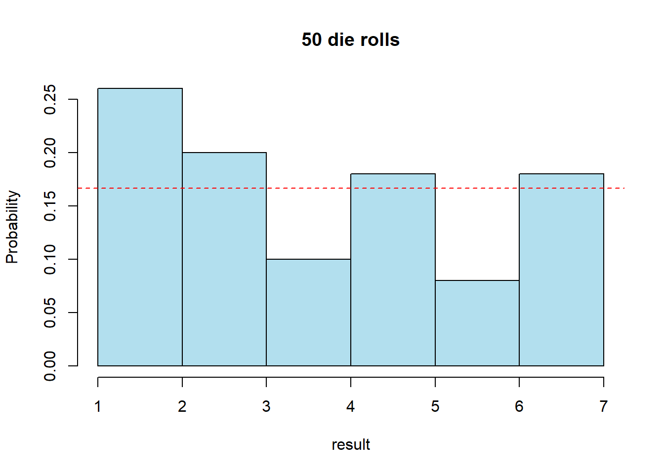
For now, we’ll define a probability distribution, similar to a histogram, but again, you should recognize that it includes (i) all possible outcomes and (ii) it shows the probability of each outcome.
What do you observe?
We know all probabilities should be equal to 1/6 = 0.1666. This value is shown above as the dashed red horizontal line. However, it doesn’t appear that all values are equally likely, nor that they all equal 0.1666. What is going on?
I include this example because it is really illustrative of the randomness that exists even when all results are equally likely, particularly for small samples.
Let’s rerun the same code, but now look at the distribution of 10000 rolls
rolls <- sample(seq(1:6), 10000, replace=T)
truehist(rolls, nbins = 6, xlab="result", ylab="Probability", main="10000 die rolls", col="lightblue2", ylim=c(0, 0.3))
abline(h=0.1666, col="red", lty=2)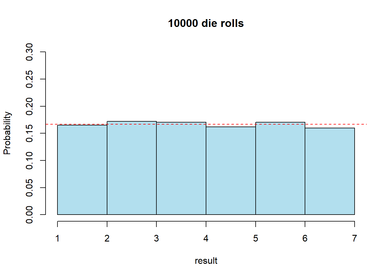
Interestingly, what we see here is that there is still some variation, however our results are much closer to the theoretical probability distributions.
This is an illustration of the “Law of Large Numbers”.
4.8 Review
| Name | Equation |
|---|---|
| Complement | \(P(A) + P(!A) = 1\) |
| For an Event with n outcomes | \(P(A_1) + P(A_2) + ... + P(A_n) = 1\) |
| Addition Rule (if Disjoint) | \(P(A\ or\ B) = P(A) + P(B)\) |
| General Addition Rule | \(P(A\ or\ B) = P(A) + P(B) - P(A\ and\ B)\) |
| Multiplication Rule for Independence | \(P(A\ and\ B) = P(A)\)*\(P(B)\) |
| Joint Probabilities | \(P(A) = P(A\ and \B) + P(A\ and\ !B)\) |
and again, these are all equations so you can manipulate as necessary based on algebraic rules.
4.8.1 Review of Learning Objectives
By the end of this chapter you should be able to:
- Define basic probability terms: probability, random variable, event, outcome, independence, disjoint, mutually exclusive, complement
- Write the relationship between events outcomes and probabilities using probability notation
- Apply logical operations OR and AND and calculate associated probabilities for simple combinations of outcomes
- Distinguish between events that are disjoint or not, and events that are independent or not
- Apply the ‘addition’ and ‘multiplication’ rules for probability and explain how the assumption of independence can be used to simplify both rules
- Define what joint and marginal probabilities are and explain where joint and marginal probabilities appear in 2x2 (or similar) contingency tables
- Calculate both joint and marginal probabilities given the appropriate information
- Demonstrate how to evaluate whether multiple events appear to exhibit independence
- Create and use a contingency table based on probabilities or counts, including converting between counts and probabilities (or proportions). Calculate and fill in missing values. Interpret the various cells.
Additionally, using R you should be able to
- Simulate discrete random data using the
sample()function, including creating the full set using theseq()andc()functions - Differentiate between sampling with and without replacement
- Define and plot what a probability distribution is
- Understand how simulation can help illustrate the “Law of Large Numbers”
4.9 Summary of R functions in this Chapter
| function | description |
|---|---|
sample() |
to generate a random sample of from a discrete data set |
seq() |
to create vector that is a sequence of consecutive numbers |
library() |
to load an external library, may contain functions and data |
vector() |
to create an empty storage vector |
truehist() |
from the MASS library, a better way to draw histograms |
for(var in seq) |
a control-flow construct to run a specified number of times |
4.10 Exercises
Note: These are not required and will occasionally be used during class as warm-up exercises or no-stakes quizzes.
Exercise 4.1 Assuming a well shuffled, fair 52 card deck, answer the following. Let H be the event of drawing a Heart and Q be the event of drawing a Queen. Use appropriate probability notation.
- What is the probability of drawing a Heart? What is the probability of drawing a Queen?
- What is the probability of drawing a Heart or a Queen?
- What is the probability of drawing a Heart and a Queen?
- Is drawing a Heart and a Queen disjoint? Is drawing a heart and a Queen independent? Explain why or why not.
Exercise 4.2 With rolling two fair six sided dice, answer the following. Use appropriate probability notation. Hint: You may find it useful to draw a 6x6 table.
- What is the probability of rolling at least one 3?
- What is the probability of rolling exactly one even number?
- What is the probability that the first die is greater than the second die?
Exercise 4.3 With rolling two four sided dice, answer the following. Use appropriate probability notation.
- What are all the possible outcomes of the sum of two dice? Are each of these outcome equally likely?
- What is the probability of getting a sum equal to 7?
- Now, calculate the probabilities of all the possible outcomes of the sum of two dice.
- Based on (c), what is the probability of getting a sum greater than or equal to 4?
- What is the probability of getting a sum less than or equal to 3? How is your answer to (d) related mathematically to your answer to here?
Exercise 4.4 For each of the following pairs of events, explain whether they might reasonably be expected to be (i) independent or (ii) mutually exclusive? If you don’t think they’re independent, explain what type of relationship you’d expect to occur. Justify your answer with 1 or 2 sentences.
- whether the Seahawks or Sounders make the playoffs this year
- whether a student takes a gap year and their academic success in college
- the weather on successive days
- a student’s test scores in math and history
- the success of a university’s sports program and their academic rigor
- carbon emissions (by country) and that country’s GDP
Exercise 4.5 The following table shows the interaction between two events G and H. Does this table suggest these events are independent? Why or why not?
| prob | G | !G |
|---|---|---|
| H | 0.1 | 0.15 |
| !H | 0.3 | 0.45 |
Exercise 4.6 Caroline has a 50% chance of receiving an A grade in History, a 34% chance of receiving an A grade in Calculus and a 10% chance of receiving A grades in both.
- Let H be the event she gets an A in History and C be the event she gets an A in Calculus. What are \(P(H)\), \(P(C)\) and \(P(H\ and\ C)\)?
- Find the probability that she receives an A in History OR Calculus.
- Create and fill in the 2x2 table showing all probabilities.
- Are these grades independent of one another?
Exercise 4.7 Given events G and H where \(P(G) = 0.43\), \(P(H) = 0.26\), and \(P(G\ and\ H) = 0.14\).
- Create the 2x2 table showing all of the joint probabilities.
- Find \(P(G\ or\ H)\).
- Find \(P(G\ and\ !H)\)
- How would you write the complement of the event (G AND H). What is it’s probability?
- How would you write the complement of the event (G OR H). What is it’s probability?
Exercise 4.8 Data from EPS suggest that each year, 25% of students miss exactly 1 day of school, 15% miss 2 days and 28% miss 3 or more days of school due to sickness.
- What is the probability that a student chosen at random does not miss any days of school due to sickness this year?
- What is the probability that a student chosen at random misses no more than one day?
- What is the probability that a student chosen at random misses at least one day?
- If a parent has two kids at EPS, what is the probability that neither student will miss any school? Note any assumptions you make.
- If a parent has two kids at EPS, what is the probability that both kids will miss some school, i.e. at least one day? Note any assumption you make.
Exercise 4.9 Assume probabilities of events \(C\) and \(D\) are known (and written as \(P(C)\) and \(P(D)\), respectively). Also assume events C and D are mutually exclusive. Write all answers in terms of C and D.
- What is the probability of \(P(C\ OR\ D)\)?
- What is the probability of \(P(C\ AND\ !D)\)?
- Is the \(P(!C\ AND\ !D)\) knowable? (As a hint, think about events that could occur from rolling a single die.)
Exercise 4.10 A Pew Research study asked 2,373 randomly sampled registered voters about (i) their political affiliation (Republican/Democrat or Independent) and (ii) whether or not they identify as swing voters (i.e. someone who votes more for policies than politicians). 35% of respondents identified as Independent, 23% identified as swing voters, and 11% identified as both.
- Are being Independent and being a swing voter disjoint (i.e. mutually exclusive)?
- What percent of voters are Independent but not swing voters?
- What percent of voters are independent or swing voters?
- Create a the 2x2 contingency table to show all joint and marginal probabilities.
- Is the event that someone is a swing voter independent of the event that someone is a political Independent?
Exercise 4.11 The table below shows the distribution of education level attained by US residents by gender based on data collected in the 2010 American Community Survey.
- Fill in the missing values. What do the numbers in each column represent?
- What is the probability that a randomly chosen female has a graduate or professional degree as the highest education level attained?
- What is the probability that a randomly chosen male has a Bachelor’s degree as the highest education level attained?
- What is the probability that a randomly chosen male has no more than a HS graduate or equivalent?
- What is the probability that a randomly chosen female has at least some college?
| Highest Education attained | Male | Female |
|---|---|---|
| Less than 9th grade | 0.07 | 0.13 |
| 9th to 12th grade, no diploma | 0.10 | 0.09 |
| HS graduate (or equivalent) | 0.30 | 0.20 |
| Some college, no degree | 0.22 | |
| Associate’s degree | 0.06 | 0.08 |
| Bachelor’s degree | 0.17 | |
| Graduate or professional degree | 0.09 | 0.09 |
Exercise 4.12 Suppose that 78% of the students at a particular college have a Facebook account and 43% have a Twitter account.
- Using only this information, what is the largest possible value for the percentage who have both a Facebook account and a Twitter account? Describe the (unrealistic) situation in which this occurs.
- Using only this information, what is the smallest possible value for the percentage who have both a Facebook account and a Twitter account? Describe the (unrealistic) situation in which this occurs.
Now assume that 36% of the students have both a Facebook account and a Twitter account.
- What percentage of students have at least one of these accounts?
- What percentage of students have neither of these accounts?
- What percentage of students have one of these accounts but not both?
(From Allan Rossman)
Exercise 4.13 When playing Minecraft if you kill a Skeleton, it randomly drops between 0-2 “arrows” and between 0-2 “bones”. Imagine you played Minecraft for a while and killed 50 skeletons with the following results of drops:
| number | 0 bones | 1 bone | 2 bones |
|---|---|---|---|
| 0 arrows | 6 | 5 | 5 |
| 1 arrow | 4 | 7 | 6 |
| 2 arrows | 6 | 4 | 6 |
- What are the total number of arrows you received? What are the total number of bones you received?
- What are all of the observed marginal and joint probabilities? What do your joint probabilities sum to?
- What is the probability of a drop of no bones or arrows? Make sure to write this in appropriate probability notation.
- What is the probability of seeing 2 arrows or 2 bones? Make sure to write this in appropriate probability notation.
- Based on this data, do you think the drops of arrows and bones are independent?
Exercise 4.14 Assume a deck with 51 cards(something is missing!) Can you figure out which? You are given the following information:
- \(P(diamond) = \frac{13}{51}\)
- \(P(face) != P(2...4)\)
- \(P(5\ or\ red) < P(6\ or\ black)\)
- \(P(even\ and\ diamond) = P(even\ and\ heart)\)
- \(P(!J) = P (!K)\)
Can you identify the missing card?
4.10.1 Simulation
Exercise 4.15 Simulate the sum of rolling three (3) six-sided die. Does it matter if you sample with or without replacement? Why or why not? How might you do this without setting the number of trials to 3?
Exercise 4.16 Simulate counting the number of heads seen when flipping a coin 6 times. (Hint, use table())
- Does it matter if you sample with or without replacement? Why or why not?
- Calculate the observed probability of success, \(\hat p\).
- Now change the probabilities so it is no longer a fair coin and repeat. How closely does your \(\hat p\) track the true value?
Exercise 4.17 In section 4.5 code was given to simulate the roll of two six sided dice and calculate the sum.
- Modify that code to run 1000 samples.
- Create a well labeled histogram of your results, using the
truehist()function. Comment on the shape of the distribution.
Exercise 4.18 Simulate the distribution of the maximum of rolling two six sided die. Use a for{} loop. b. Create a well labeled histogram of your results, using the truehist() function. Comment on the shape of the distribution.
Exercise 4.19 Imagine a situation where you have a bowl with 5 different colored Skittles, but not in equal probabilities. Let’s assume the bowl contains 6 Yellow, 5 Orange, 6 Red, 3 Green and 4 Purple candies.
What is the maximum number you can draw without replacement (if there is one)? What is the maximum number you can draw with replacement (if there is one)?
Using the
sample()function, write a short bit of R code to simulate drawing 12 candies from the bowl, without replacement. (Hint: be careful about creating your full sample. Maybe therep()function is useful?) Then use thetable()function to count the results of each candy. Print out an example.Use the
barplot()function on thetable()results to plot the probability distribution of a single draw. However, this isn’t quite right because of our y axis. Instead, create a histogram oftable()/12(since you sampled 12 candies) of course putting the appropriate variable within the parenthesis.Is your plot from (c) representative of the true probabilities of drawing different candy colors? Why or why not?
Exercise 4.20 (CHALLENGING!) Continuing with the above example, we will now use simulation to look at the distribution of how many Yellow candies we could draw (out of 12).
- First, we need to extract counts from our simulated results. Suppose you had a color “X” and your sample was stored in variable
a, you could usetable()but it doesn’t do well when the are 0 results for a given color. Instead, inspect the following code:
Explain what this code does and verify that it works correctly.
- Let’s now simulate the probability of drawing 0, 1, 2 … yellow candies. You’ll use a
for{}loop to run 10,000 simulations. Some scaffolding is provided below. Fill in the for loop as necessary to store the results from each simulation.
## Create storage for the simulations
rslt <- vector("numeric", 10000)

for (i in 1:10000) {
  ## Take a single sample of 12 candies

  ## Extract the number of Yellow.

  ## Store the value in the rslt vector
  rslt[i] <- ...
}

## plot a histogram of the rslt vector- Add code to plot a histogram of the
rsltvector as shown on the last line. Is this a probability distribution, why or why not?